Note

This page was generated from tut/4-Analysis/pyaedt-multiplanar/Eigenmode-pyaedt-multiplanar.ipynb.

Running Eigenmode Simulations & EPR Analysis with QHFSSEigenmodePyaedt

This notebook is a tutorial on how to use QHFSSEigenmodePyaedt class.

First, what is an eigenmode solver? “The eigenmode solver is used to calculate the frequencies and the corresponding electromagnetic field patterns (eigenmodes), when no excitation is applied.” From MIT - Eigenmode Solver Overview.

This is all fine, but our circuit contains quantum effects and Ansys uses a purely classical electromagnetic solver. How can we predict qubit anharmonicity and dispersive shift? Well, we can use Energy Participation Ratio (EPR) analysis to quantize the circuit. Luckily for us, Quantum Metal integrates pyEPR, allowing for easy implementation of EPR analysis.

This notebook simulates a single transmon qubit and runs EPR analysis on it.

💡 Desktop GUI or inline. metal.gui(design) opens the desktop MetalGUI when Qt and a display are available and falls back to an inline viewer (Colab, Binder, a server) with the same API, so gui.rebuild() and gui.screenshot() work in both. See 1.1 Quick start and `docs/headless-usage.rst <https://qiskit-community.github.io/qiskit-metal/headless-usage.html>`__.

The design and its screenshot run anywhere. From “Launch eigenmode analysis” on, the cells drive Ansys HFSS through pyaedt and pyEPR; they need Ansys Electronics Desktop and are shown here without outputs.

🧭 Other simulation pathways. This notebook uses Ansys, which needs a license. Without one, the same kind of result can come from the open-source ElmerFEM path for capacitance (tutorial 4.19) or the pip-installable gmsh + scikit-fem solver for eigenmodes, couplings and capacitance (tutorials 4.43–4.45); AWS Palace is available through SQDMetal, with a native integration in progress. Simulation pathways summarizes what each solver computes, how to install it, and which tutorials use it.

import qiskit_metal as metal
from qiskit_metal.designs.design_multiplanar import MultiPlanar
from qiskit_metal.qlibrary.qubits.transmon_cross import TransmonCross
from qiskit_metal.renderers.renderer_ansys_pyaedt.hfss_renderer_eigenmode_aedt import (
    QHFSSEigenmodePyaedt,
)

Use Multiplanar design, for Ansys HFSS Eigenmode simulation using pyaedt renderer

DISCLAIMER: For now, this might only work with the full version (paid) of Ansys and not the student version. This issue is fixable and requires more testing. Please run the notebook and test it out on student license, if you’re interested to make a contribution!

design = MultiPlanar(metadata={}, overwrite_enabled=True)

# Check if layer data is usable, if so launch GUI
ls_unique = design.ls.is_layer_data_unique()
if not ls_unique:
    raise ValueError("Layer data in `MultiPlanar` design is not unique")

gui = metal.gui(design)

A single transmon

Create the design

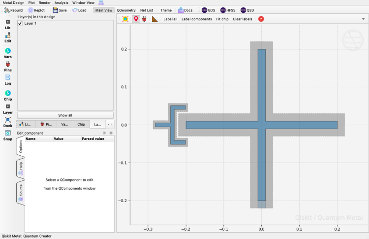
The design is a single Xmon-style transmon with one readout pad.

xmon_options = dict(
    connection_pads=dict(readout=dict()),
)

TransmonCross(design, "transmon", options=xmon_options)

gui.rebuild()
gui.zoom_on_components(["transmon"])
gui.screenshot()

Launch eigenmode analysis

This uses pyaedt to connect to Ansys. As of May 2023 only the paid version of Ansys was supported.

em1_aedt = QHFSSEigenmodePyaedt(
    design, "Eigenmode_Tutorial", "Qubit ONLY", initiate=True
)

# Path to access Hfss pyAEDT object
hfss_aedt = em1_aedt.current_app

Render Design to ANSYS

em1_aedt.render_design()

Add Setup

To create a setup in ANSYS, we call the method add_hfss_em_setup, it has the arguments:

Create a solution setup in Ansys HFSS Driven-Modal solution type. If user does not provide
        arguments, they will be obtained from QHFSSDrivenmodalPyaedt.default_setup dict.

        Args:
            name (str, optional): _description_. Defaults to None.
            MinimumFrequency (float, optional):  Minimum frequency in GHz. Defaults to self.default_setup.
            NumModes (int, optional): Number of modes.  Defaults to self.default_setup.
            MaxDeltaFreq (float, optional):   Maximum difference in freq between consecutive passes.
                                        Defaults to self.default_setup.
            MaximumPasses (int, optional):  Maximum number of passes. Defaults to self.default_setup.
            MinimumPasses (int, optional): Minimum number of passes.Defaults to self.default_setup.
            MinimumConvergedPasses (int, optional): Minimum number of converged passes.
                                        Defaults to self.default_setup.
            PercentRefinement (int, optional): Percent refinement. Defaults to self.default_setup.
            BasisOrder (int, optional): Basis order. Defaults to self.default_setup.

        Returns:
            new_setup (pyaedt.modules.SolveSetup.SetupHFSS): pyAEDT simulation setup object.

In Eigenmode simulations, we can directly find the resonant frequency. This is in comparison to a DrivenModal simualtion, where we need to sweep the frequency space and find the resonant response.

Since the transmon has a resonant frequency, we are ONLY simulating a transmon. We have 1 resonant mode. Hence NumModes = 1.

setup_name = "Setup_QubitONLY"

# Add Setup
setup_options = dict(
    name=setup_name,
    MinimumFrequency=3,  # GHz
    NumModes=1,  # THIS IS ONLY FOR A SINGLE TRANSMON
    MaxDeltaFreq=0.1,
    MaximumPasses=5,
    MinimumPasses=1,
    MinimumConvergedPasses=2,
    PercentRefinement=30,
    BasisOrder=None,
)

em1_aedt.add_hfss_em_setup(**setup_options)

Analyze Setup (run ANSYS simulation)

em1_aedt.analyze_setup(setup_name)

Run EPR Analysis

From here, we use pyEPR to run the EPR analysis.

Format of results:
    f_0 [MHz]    : Eigenmode frequencies computed by HFSS; i.e., linear freq returned in GHz
    f_1 [MHz]    : Dressed mode frequencies (by the non-linearity; e.g., Lamb shift, etc. ).
                    If numerical diagonalizaiton is run, then we return the numerically diagonalizaed
                    frequencies, otherwise, use 1st order pertuirbation theory on the 4th order
                    expansion of the cosine.
    f_ND [MHz]   : Numerical diagonalizaiton
    chi_O1 [MHz] : Analytic expression for the chis based on a cos trunc to 4th order, and using 1st
                    order perturbation theory. Diag is anharmonicity, off diag is full cross-Kerr.
    chi_ND [MHz] : Numerically diagonalized chi matrix. Diag is anharmonicity, off diag is full
                    cross-Kerr.

Args:
    cos_trunc (int, optional): Truncation of the cosine. Defaults to 8.
    fock_trunc (int, optional): Truncation of the fock. Defaults to 7.
    print_results (bool, optional): Print results of EPR analysis. Defaults to True.
    numeric (bool, optional): Use numerical diagonalization. Defaults to True.

    Returns:
        self.epr_quantum_analysis.data (dict): all results of EPR analysis

epr_data = em1_aedt.run_epr(print_result=True)

print(epr_data)

For more information, review the Introduction to Quantum Computing and Quantum Hardware lectures below

Superconducting Qubits I: Quantizing a Harmonic Oscillator, Josephson Junctions Part 1	Lecture Video	Lecture Notes	Lab
Superconducting Qubits I: Quantizing a Harmonic Oscillator, Josephson Junctions Part 2	Lecture Video	Lecture Notes	Lab
Superconducting Qubits I: Quantizing a Harmonic Oscillator, Josephson Junctions Part 3	Lecture Video	Lecture Notes	Lab
Superconducting Qubits II: Circuit Quantum Electrodynamics, Readout and Calibration Methods Part 1	Lecture Video	Lecture Notes	Lab
Superconducting Qubits II: Circuit Quantum Electrodynamics, Readout and Calibration Methods Part 2	Lecture Video	Lecture Notes	Lab
Superconducting Qubits II: Circuit Quantum Electrodynamics, Readout and Calibration Methods Part 3	Lecture Video	Lecture Notes	Lab