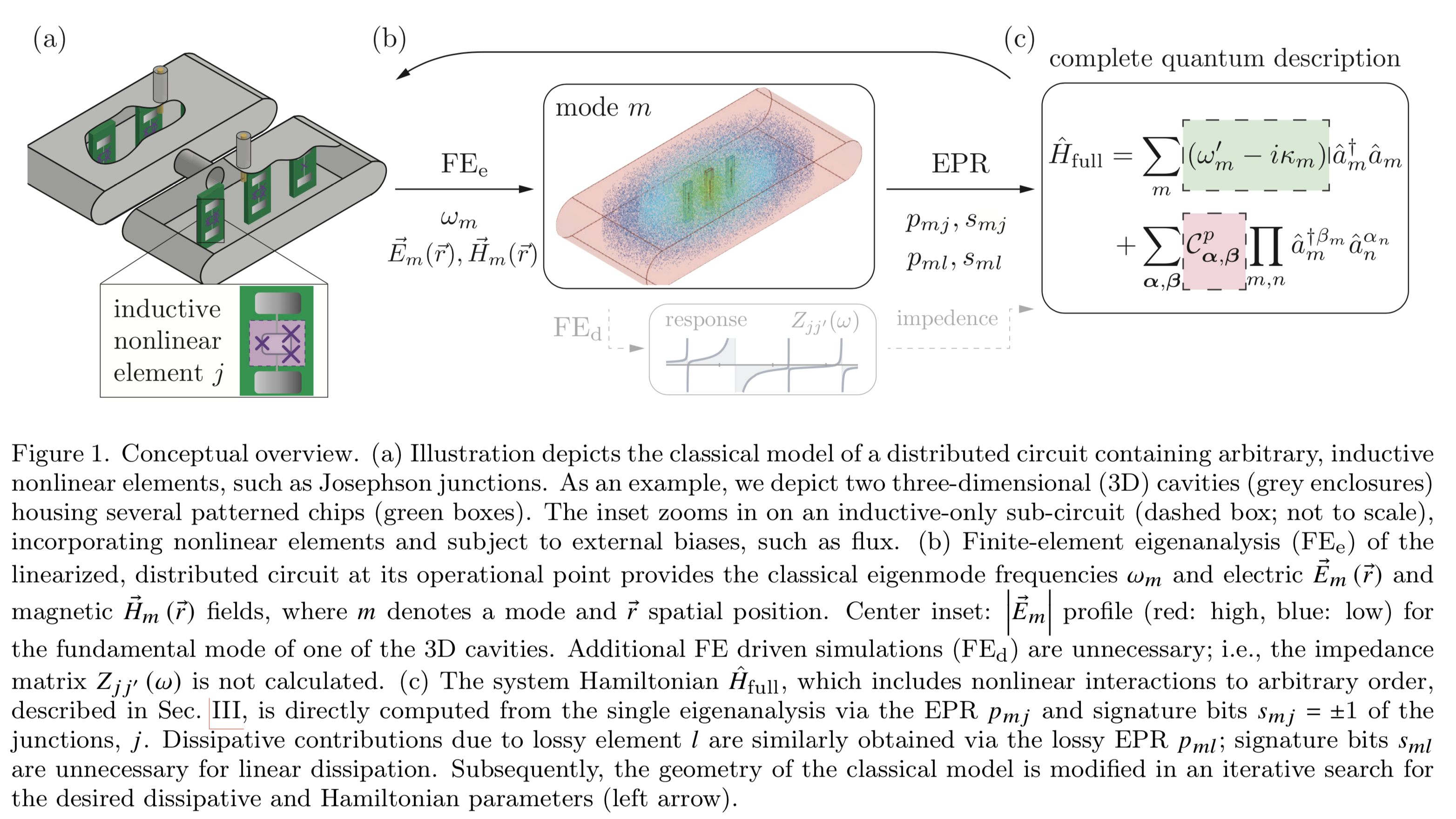
Quantization Methods Overview
We currently support two complementary quantization approaches that cover most day-to-day chip design work: a lightweight lumped/ quasi-lumped model and a full-wave, black-box style energy-participation ratio (EPR) workflow. Use this section as a quick “why and when” guide before you pick a solver.
What you give us - Your device geometry (from the QComponent library or your own components) - A small set of materials/stack assumptions (dielectrics, metal films, boundaries) - The excitation/ports you care about (for scattering or eigenmode solves)
What you get back - Modal frequencies, anharmonicities, and dispersive shifts - Coupling strengths and participation matrices you can plug into Hamiltonians - Loss estimates tied to specific volumes (dielectrics, conductors, seams) so you can chase the right bottleneck
Each method balances speed, fidelity, and required setup. Start with the lumped model when you need fast iteration and intuitive circuit pictures; switch to EPR when geometry and field participation really matter.
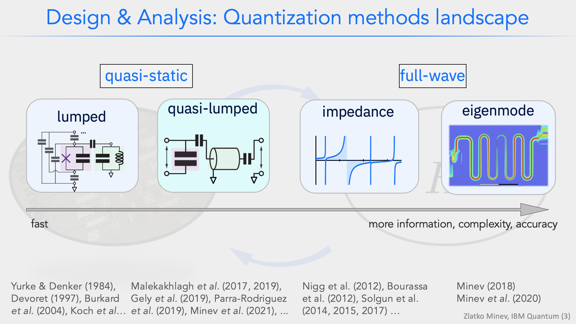
Lumped-oscillator model
In the lumped-oscillator model you treat each component as a compact circuit element whose capacitance and inductance can be extracted from fast quasi-static simulations or closed-form formulas. Think of it as a guided way to draw a circuit, pull out the C and L values, and then stitch those into a Hamiltonian.
When to use it. Early design and parameter sweeps when you want intuition and speed. Routing, connector placement, and first-order coupling strengths are often “good enough” here. Because solves are cheap, you can explore a lot of geometry/stack variants before moving to heavier solvers.
How it works. Partition the device into a handful of cells, solve each one quickly to get effective C/L values, then assemble the network and quantize. The reduction step preserves the pairwise couplings so you keep track of renormalization and loading. The result is a simple Hamiltonian with parameters you can iterate on in minutes.
References:
Zlatko K. Minev, Thomas G. McConkey, Maika Takita, Antonio Corcoles, Jay M. Gambetta, Circuit quantum electrodynamics (cQED) with modular quasi-lumped models. (2021)
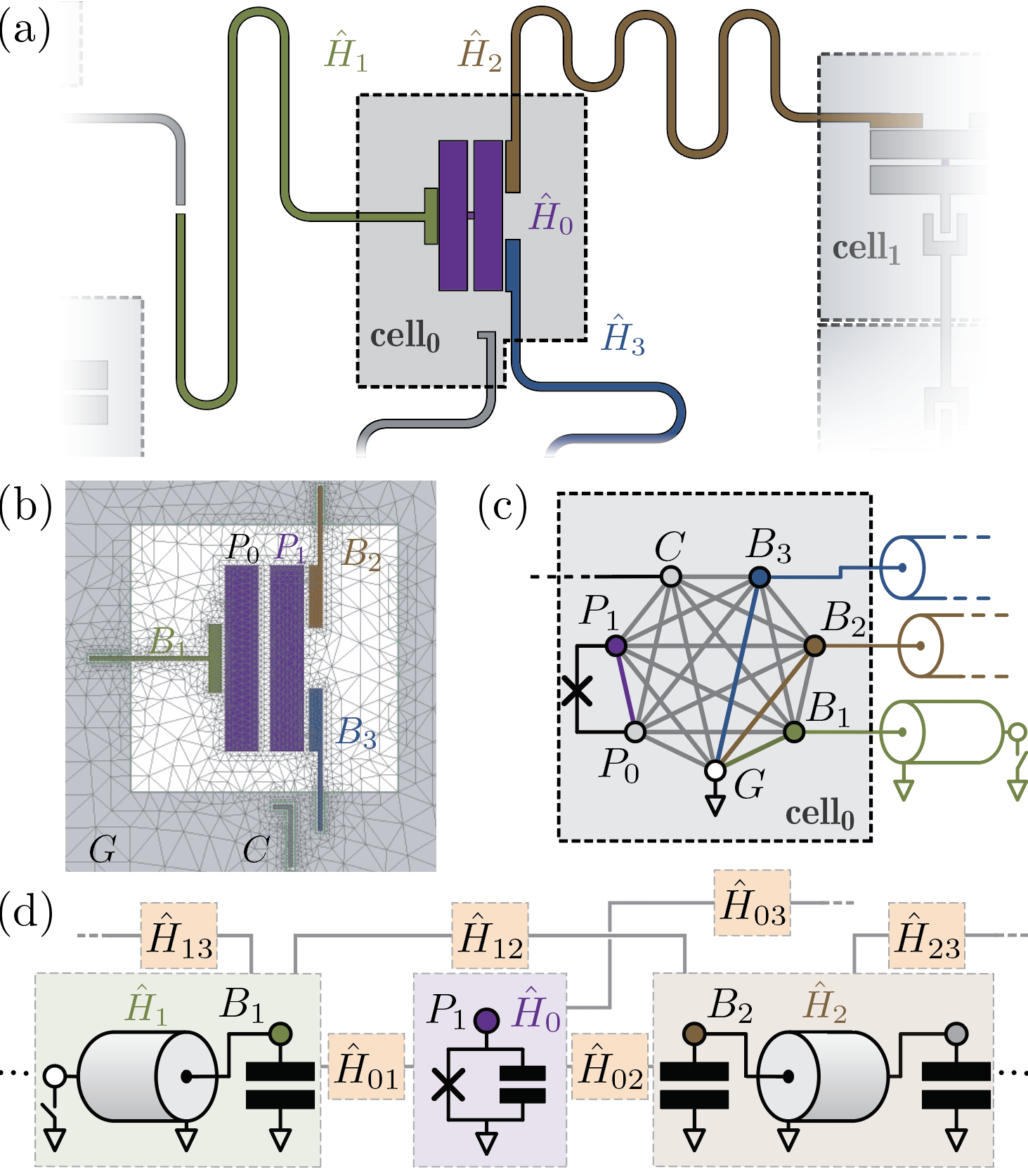
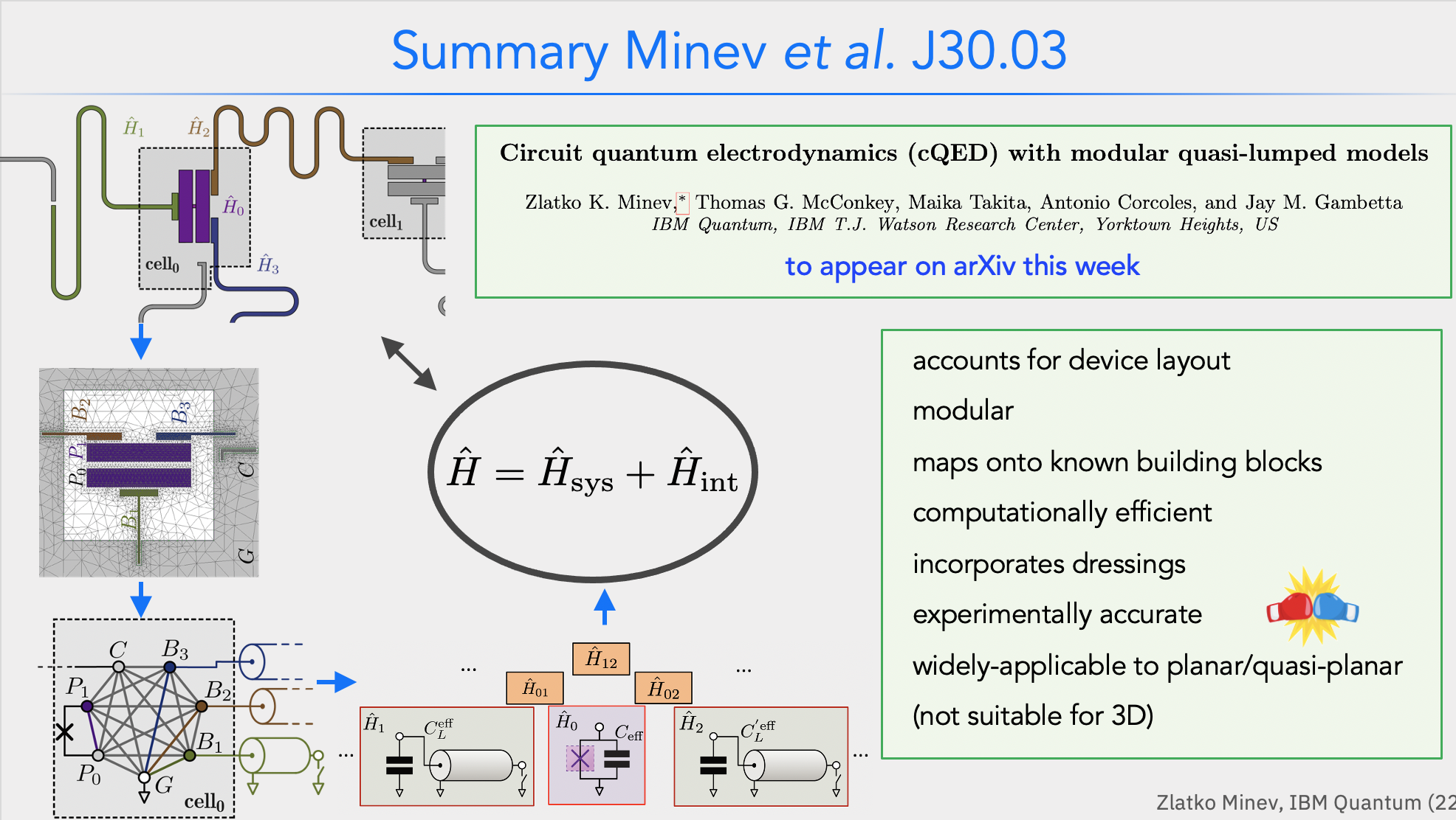
Composite-system API: Cell / Subsystem / CompositeSystem
The lumped-oscillator model is assembled from three classes in
qiskit_metal.analyses.quantization.lom_core_analysis. A Cell holds
an extracted capacitance matrix plus any inductors and junctions; a
Subsystem maps a set of circuit nodes to a quantum model (transmon,
fluxonium, transmission-line or lumped resonator, …); and a
CompositeSystem reduces and quantizes the combined network. These are the
classes used in tutorials 4.04 and 4.05.
The accepted q_opts for every built-in subsystem sys_type
(TRANSMON, FLUXONIUM, TL_RESONATOR, LUMPED_RESONATOR) — which
values you supply and which are computed from the extracted L and C matrices —
are listed on Subsystem below. Call
QuantumSystemRegistry.registry() to enumerate every registered type,
including any custom builder you add.
- class Cell(options: dict)[source]
A physical subdivision of the device (i.e., the composite system), a sub-graph of capaciators, inductoros and other linear or non-linear circuit elements. The cell can be independently simulated to extract its electromagnetic parameters, which the the user provides as inputs to this object
Initialize the cell object
- Parameters:
options (Dict) –
options can contain the following keys:
node_rename(dict): a dict mapping from original node names to new node names, {old_name: new_name}cap_mat(pd.DataFrame): Maxwell capacitance of the cell in pandas dataframeind_dict(dict): the keys are tuples of specifying the two nodes between which the inductors lie. For example, {(‘n1’, ‘n2’): 10} specifies that there is an inductor of 10 nH between node ‘n1’ and ‘n2’ for one cell and an inductor of 13 nH between node ‘n5’ and ‘n7’ for another celljj_dict(dict): dict mapping original circuit nodes to custom-named junction nodes. This is the parameter informing the LOM analysis between which nodes the Josephson junctions are located. For example, {(‘n1’, ‘n2’): ‘j1’} specifies that there is a junction between nodes ‘n1’ and ‘n2’ and named as ‘j1’cj_dict(dict): if provided, specifies the junction capacitances in each cell. Structure is the same as ind_dict. For the dict, the keys are tuples of specifying the two nodes between which the junctions lie. For example, {(‘n1’, ‘n2’): 2} specifies that there is an junction capacitance of 2 fF between node ‘n1’ and ‘n2’ for the first provided cell and None for the second provided cell.
- class Subsystem(name: str, sys_type: str, nodes: list[str], q_opts: dict = None)[source]
Class representing a subsystem that can typically be mapped to a quantum system with known solution, such as a transmon, a fluxonium or a quantum harmonic oscillator.
A subsystem is defined by three things: a
name, asys_type(which built-in or custom quantum model it maps to), and the list of circuitnodesit occupies. Type-specific numbers — offset charge, external flux, resonator frequency, scQubits truncation, etc. — are passed through theq_optsdict.Units: energies (
EJ,EL,EC) are in MHz and frequencies (f_res) are in GHz. TheTRANSMONandFLUXONIUMbuilders computeEC(and, for the transmon,EJ) in MHz, so the resulting eigenvalues are in MHz even though scqubits’ default unit label is GHz; callscqubits.set_units("MHz")for correctly labelled plots.Built-in
sys_typevalues and theirq_opts¶The list below is the accepted-parameter reference for the four models shipped with quantum-metal. Call
QuantumSystemRegistry.registry()at runtime to list every registered type, including any you have added yourself. Parameters marked (computed) are extracted from the reduced L and C matrices during the LOM solve and must not be supplied; the rest are optional and fall back to the defaults shown."TRANSMON"— maps toscqubits.Transmon.EJ,EC— (computed) from the extracted L and C matrices.ng— offset charge (default0.001).ncut— charge-basis cutoff (default22).truncated_dim— retained levels (default10).nodes— a single junction node.
"FLUXONIUM"— maps toscqubits.Fluxonium.EC— (computed) from the extracted C matrix.EJ— Josephson energy in MHz (required).EL— inductive energy in MHz (required).flux— external flux in units of the flux quantum \(\Phi_0\) (required).cutoff— basis cutoff (default110).truncated_dim— retained levels (default10).nodes— a single junction node.
"TL_RESONATOR"— distributed transmission-line resonator, maps toscqubits.Oscillator.f_res— resonator frequency in GHz (required).Z0— characteristic impedance in ohms (default50).vp— phase velocity in m/s, or the string"use_design"(default) to derive it from thedesignstack below.design— dict of the physical stack used whenvp="use_design":line_width,line_gap,substrate_thickness,film_thickness, all in meters (defaults10e-6,6e-6,750e-6,200e-9).truncated_dim— retained levels (default: chosen byCompositeSystem.create_hilbertspace(), see below).other_end_shorted—Trueif the far end is shorted to ground (defaultFalse). A shorted resonator must be given a single node.nodes— one node (open- or shorted-end) or two nodes.
"LUMPED_RESONATOR"— lumped LC resonator, maps toscqubits.Oscillator.f_res— (computed) from the extracted L and C matrices.truncated_dim— retained levels (default: chosen byCompositeSystem.create_hilbertspace(), see below).nodes— a single node.
Resonator levels. A resonator’s self-Kerr (its diagonal entry in the chi matrix) comes from its two-photon level. With only three levels that level is the top of the retained space and has no partner above it, so the self-Kerr comes out wrong (e.g. +0.57 MHz where the converged value is -0.0003 MHz); qubit frequencies, anharmonicities and qubit-resonator shifts are unaffected. When
truncated_dimis not given, resonators therefore keep 5 levels if the whole Hilbert space stays at or belowCompositeSystem.max_auto_dimensionstates, and 3 levels otherwise, with a warning that their self-Kerr is not converged.See tutorials
4.04and4.05for worked transmon / fluxonium / coupled-transmon examples.Initialize the Subsystem object
- param name:
name of the subsystem
- type name:
str
- param sys_type:
type of the subsystem. Type can be one of the types implemented by one of the concrete QuantumBuilders (call QuantumSystemRegistry.registry() to see all the choices), which can also be custom-made by user
- type sys_type:
str
- param nodes:
list of nodes the subsystem corresponds to. For example, for a transmon subsystem, this would just be a list of a single node which is the user-defined junction node in the Cell object
- type nodes:
List[str]
- param q_opts:
options relevant to the type of quantum subsystem. The Subsystem object builds the quantum subsystem using quantumfy() which calls make_quantum() of the corresponding QuantumBuilder. q_opts provides parameters needed by make_quantum(). In the case of qubit subsystems, make_quantum() takes advantage of the scQbuits package (https://scqubits.readthedocs.io). Consequently, the default options correspond to the default options of the qubit classes in scQubits. Defaults to None.
- type q_opts:
dict, optional
- property h_params
Hamiltonian parameters of the subsystem
- property quantum_system
The quantum subsystem that the subsystem corresponds to. It is built by calling an associated builder passed in quantumfy() using the Visitor pattern
- class CompositeSystem(subsystems: list[Subsystem], cells: list[Cell], grd_node: str, nodes_force_keep: Sequence = None, s_remove_provided: ndarray | bool = False, s_keep_provided: ndarray | bool = False)[source]
Class representing the composite system which may consist of multiple subsystems and cells.
A composite system stitches one or more
Cellobjects (each carrying an extracted capacitance matrix, and optionally inductors and junctions) together with theSubsystemobjects that describe which quantum model each set of nodes maps to. CallingcircuitGraph()reduces the combined L and C matrices;create_hilbertspace()andhamiltonian_results()then build and diagonalize the coupled Hamiltonian.Example
from qiskit_metal.analyses.quantization.lom_core_analysis import (
    Cell, Subsystem, CompositeSystem)

# A cell holds the extracted capacitance matrix plus the junction
cell = Cell(dict(node_rename={},
                 cap_mat=cap_df,               # pandas DataFrame
                 ind_dict={('pad_top', 'pad_bot'): 12.0},   # nH
                 jj_dict={('pad_top', 'pad_bot'): 'j1'}))

transmon = Subsystem(name='Q1', sys_type='TRANSMON', nodes=['j1'])

composite = CompositeSystem(
    subsystems=[transmon],
    cells=[cell],
    grd_node='ground',
    nodes_force_keep=None,
)
hilbertspace = composite.create_hilbertspace()
results = composite.hamiltonian_results(hilbertspace, evals_count=10)
Initialize the CompositeSystem object
- Parameters:
subsystems (List[Subsystem]) – list of Subsystem objects
cells (List[Cell]) – list of Cell objects
grd_node (str) – name of the ground node
nodes_force_keep (Sequence, optional) – a list of nodes that will not be eliminated during L and C matrices reduction. Use this parameter to specify non-dynamic nodes (nodes that are connected capacitors only or inductors only) that should be preserved. If not specified (i.e., None), all non-dynamic nodes are eliminated
s_remove_provided (np.ndarray) – precalculated s_remove; see documentation on CircuitGraph.S_Remove
s_keep_provided (np.ndarray) – precalculated s_keep; see documentation on CircuitGraph.S_Keep
- add_interaction(gs: ndarray = None, gscale: float = 1.0) HilbertSpace[source]
add interaction terms to the composite hilbertspace
- Parameters:
gs (np.ndarray) – coupling strength matrix. If not provided, it will be calculated by compute_gs()
gscale (float) – coupling strength scale
- Returns:
- Hilbertspace object for the Hamiltonian
of the composite system with interations added
- Return type:
scq.HilbertSpace
- circuitGraph() CircuitGraph[source]
create a CircuitGraph object with circuit parameters of the composite system
- Returns:
CircuitGraph object for LOM analysis
- Return type:
CircuitGraph
- compute_gs(coupling_type: str = 'CAPACITIVE')[source]
compute g matrices from reduced C inverse matrix C^{-1}_{k} and reduced L inverse matrix L^{-1}_{k} and zero point flucuations (Q_zpf, Phi_zpf)
Note that the computed g’s are in MHz
Note: the resulting matrix is in the basis of nodes_keep, which may not be in the same order of subsystems
- create_hilbertspace() HilbertSpace[source]
- create the composite hilbertspace including all the subsystems. Interaction
NOT included
Resonators without an explicit
truncated_dimget 5 levels when the whole space stays withinmax_auto_dimensionstates, else 3 (seeSubsystem, “Resonator levels”).- Returns:
- Hilbertspace object for the Hamiltonian
of the composite system without interations added
- Return type:
scq.HilbertSpace
- hamiltonian_results(hilbertspace: HilbertSpace, evals_count=None, print_info=True) dict[source]
Print and return results
- Parameters:
- Returns:
{"fQ_in_Ghz": {subsystem name: f01 in GHz}, "chi_in_MHz": LabeledNdarray of the chi matrix in MHz}- Return type:
- max_auto_dimension = 4000
Largest Hilbert space (number of states) for which resonators without an explicit
truncated_dimget 5 levels instead of 3; full dense diagonalization stays within seconds up to about this size.
Energy: The energy-participation-ratio (EPR) method
The energy-participation-ratio (EPR) method is a general (black-box) quantization method. Based on the Quantum Metal integration with pyEPR, one can automate the design and quantization of Josephson quantum circuits, and even 3D circuits.
The EPR method is based on the energy-participation ratio (EPR) of a dissipative or nonlinear element in an electromagnetic mode. The EPR, a number between zero and one, quantifies how much of the energy of a mode is stored in each element. It obeys universal constraints—valid regardless of the circuit topology and nature of the nonlinear elements. The EPR of the elements are calculated from a unique, efficient electromagnetic eigenmode simulation of the linearized circuit, including lossy elements. Their set is the key input to the determination of the quantum Hamiltonian of the system. The method provides an intuitive and simple-to-use tool to quantize multi-junction circuits. It is especially well-suited for finding the Hamiltonian and dissipative parameters of weakly anharmonic systems, such as transmon qubits coupled to resonators, or Josephson transmission lines. The EPR method is experimentally tested on a variety of Josephson circuits, and demonstrated high agreement for nonlinear couplings and modal Hamiltonian parameters, over many order of magnitude in energy.
When to use it. When layout details matter: packaging effects, higher-mode participation, junction placement, seams, or substrate losses. EPR gives you a field-aware Hamiltonian and ties every loss number to a physical volume, so you know which lever to pull next.
What you set up. Draw your design, define materials and boundaries, place ports, and run a single eigenmode solve on the linearized circuit. pyEPR reads the fields, computes participations for every nonlinear/lossy element, and hands back frequencies, dispersive shifts, anharmonicities, and loss budgets. Because it is black-box, it scales to multi-mode, multi-junction systems with minimal hand-tuning.
References:
Minev, Z. K., Leghtas, Z., Mudhada, S. O., Reinhold, P., Diringer, A., & Devoret, M. H. (2018). pyEPR: The energy-participation-ratio (EPR) open-source framework for quantum device design.
Minev, Z. K., Leghtas, Z., Mundhada, S. O., Christakis, L., Pop, I. M., & Devoret, M. H. (2020). Energy-participation quantization of Josephson circuits. ArXiv. Retrieved from http://arxiv.org/abs/2010.00620 (2020)
Z.K. Minev, Ph.D. Dissertation, Yale University (2018), Chapter 4. arXiv:1902.10355 (2018)
Impedance: impedance-based black-box quantization (BBQ)
The impedance formulation of black-box quantization builds the Hamiltonian directly from the frequency-dependent impedance seen between nonlinear elements and ground. It shares the “full-wave fields first, circuit later” philosophy of EPR, but works in the impedance domain: from a port-defined impedance matrix you extract effective mode frequencies, participation factors, and couplings.
When to use it. For strongly multi-port/multi-mode layouts where port impedances are the most natural handle (e.g., rich bus networks, Purcell filters, or chip-package assemblies). It is also a good cross check to EPR when you want to validate couplings via an independent pipeline.
What you set up. Define ports at the locations of junctions or pins, run an eigenmode or driven solve to obtain the impedance matrix versus frequency, then sample around the modes of interest. The resulting impedances map to effective inductive/capacitive participations and give you the Hamiltonian parameters.
Outputs. Mode frequencies, nonlinear participation, and cross-Kerr rates derived from the impedance matrix, plus a clear picture of how design changes move those impedances. Use it to tune Purcell filters, set coupling windows, or debug unexpected mode crowding.