Note
This page was generated from tut/4-Analysis/4.05-New-LOM-and-Two-Coupled-Transmon-Example.ipynb.
4.05 New LOM and Two Coupled Transmon Example
💡 Using this tutorial without the Qt GUI
This tutorial uses the desktop
MetalGUI. To follow along on Colab, Binder, JupyterHub, or any environment where Qt isn’t available, replace any ``gui.rebuild()`` / ``gui.screenshot()`` call with ``qm.view(design)`` — it renders the design to a matplotlibFigureyou can display inline or save withfig.savefig(...).See 1.1 Quick start for a complete runnable walkthrough and
`docs/headless-usage.rst<../../../docs/headless-usage.rst>`__ for the full reference.
[3]:
QuantumSystemRegistry.registry()
[3]:
{'TRANSMON': qiskit_metal.analyses.quantization.lom_core_analysis.TransmonBuilder,
 'FLUXONIUM': qiskit_metal.analyses.quantization.lom_core_analysis.FluxoniumBuilder,
 'TL_RESONATOR': qiskit_metal.analyses.quantization.lom_core_analysis.TLResonatorBuilder,
 'LUMPED_RESONATOR': qiskit_metal.analyses.quantization.lom_core_analysis.LumpedResonatorBuilder}
Example: two transmons coupled by a direct coupler
1. load transmon cell Q3d simulation results
Loading the Maxwell capacitance matrices for the design as shown in the screenshot below:
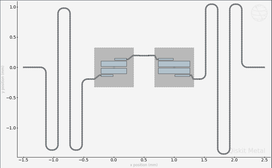
where we have two transmons (alice and bob) coupled to each other through a direct coupler. Each transmon is also coupled to its own readout reasonator.
For a simple introduction on Maxwell capacitance matrix, check out the following resources: https://www.fastfieldsolvers.com/Papers/The_Maxwell_Capacitance_Matrix_WP110301_R02.pdf
[4]:
# loading alice's simulation results
path1 = "./Q1_TwoTransmon_CapMatrix.txt"
ta_mat, _, _, _ = load_q3d_capacitance_matrix(path1)
Imported capacitance matrix with UNITS: [fF] now converted to USER UNITS:[fF]                 from file:
        ./Q1_TwoTransmon_CapMatrix.txt
| coupler_connector_pad_Q1 | ground_main_plane | pad_bot_Q1 | pad_top_Q1 | readout_connector_pad_Q1 | |
|---|---|---|---|---|---|
| coupler_connector_pad_Q1 | 59.20 | -37.28 | -2.01 | -19.11 | -0.23 |
| ground_main_plane | -37.28 | 246.33 | -39.79 | -39.86 | -37.30 |
| pad_bot_Q1 | -2.01 | -39.79 | 93.05 | -30.61 | -19.22 |
| pad_top_Q1 | -19.11 | -39.86 | -30.61 | 92.99 | -2.01 |
| readout_connector_pad_Q1 | -0.23 | -37.30 | -19.22 | -2.01 | 59.33 |
[5]:
# loading bob's simulation results
path2 = "./Q2_TwoTransmon_CapMatrix.txt"
tb_mat, _, _, _ = load_q3d_capacitance_matrix(path2)
Imported capacitance matrix with UNITS: [fF] now converted to USER UNITS:[fF]                 from file:
        ./Q2_TwoTransmon_CapMatrix.txt
| coupler_connector_pad_Q2 | ground_main_plane | pad_bot_Q2 | pad_top_Q2 | readout_connector_pad_Q2 | |
|---|---|---|---|---|---|
| coupler_connector_pad_Q2 | 64.52 | -38.63 | -2.18 | -22.93 | -0.22 |
| ground_main_plane | -38.63 | 267.40 | -49.28 | -49.30 | -38.67 |
| pad_bot_Q2 | -2.18 | -49.28 | 121.38 | -45.24 | -23.06 |
| pad_top_Q2 | -22.93 | -49.30 | -45.24 | 121.24 | -2.18 |
| readout_connector_pad_Q2 | -0.22 | -38.67 | -23.06 | -2.18 | 64.70 |
2. Create LOM cells from capacitance matrices
Setting cell objects corresponding to the capacitance simulation results
coupler_connector_pad_Q1 and coupler_connector_pad_Q2 refer to the same node corresponding to the direct coupler between the qubits but are different names in the capacitance matrix results file. In order to merge the two capacitance matrices in the LOM analysis, we need to rename them to be the same name. Also renaming readout_connector_pad_Q1 and readout_connector_pad_Q2 for clarity’s sake.
The following three parameters, ind_dict, jj_dict, cj_dict, all have the same structure. Each is a dictionary where the keys are tuples, giving the nodes that a junction is in between, and the values specifying the relevant values associated with the junction. ind_dict lets you specify the junction inductance in nH; jj_dict specifies the Josephson junction name (you can give the junction any name you wish; just need to be consistent with the name); cj_dict specifies the
junction capacitance in fF.
[6]:
# cell 1: transmon Alice cell

opt1 = dict(
    node_rename={
        "coupler_connector_pad_Q1": "coupling",
        "readout_connector_pad_Q1": "readout_alice",
    },
    cap_mat=ta_mat,
    ind_dict={("pad_top_Q1", "pad_bot_Q1"): 10},  # junction inductance in nH
    jj_dict={("pad_top_Q1", "pad_bot_Q1"): "j1"},
    cj_dict={("pad_top_Q1", "pad_bot_Q1"): 2},  # junction capacitance in fF
)
cell_1 = Cell(opt1)


# cell 2: transmon Bob cell
opt2 = dict(
    node_rename={
        "coupler_connector_pad_Q2": "coupling",
        "readout_connector_pad_Q2": "readout_bob",
    },
    cap_mat=tb_mat,
    ind_dict={("pad_top_Q2", "pad_bot_Q2"): 12},  # junction inductance in nH
    jj_dict={("pad_top_Q2", "pad_bot_Q2"): "j2"},
    cj_dict={("pad_top_Q2", "pad_bot_Q2"): 2},  # junction capacitance in fF
)
cell_2 = Cell(opt2)
3. Create subsystems
Creating the four subsystems, corresponding to the 2 qubits and the 2 readout resonators
Subsystem takes three required arguments. The four currently supported system types are TRANSMON, FLUXONIUM, TL_RESONATOR (transmission line resonator) and LUMPED_RESONATOR. nodes lets you specify which node the subsystem should be mapped to in the cells. They should be consistent with the node names you have given previously. q_opts lets specify any optional parameters you want to give. For example, for qubits, you can provide scqubits parameters such as
ncut, truncated_dim here.
[7]:
# subsystem 1: transmon Alice
transmon_alice = Subsystem(name="transmon_alice", sys_type="TRANSMON", nodes=["j1"])


# subsystem 2: transmon Bob
transmon_bob = Subsystem(name="transmon_bob", sys_type="TRANSMON", nodes=["j2"])


# subsystem 3: Alice readout resonator
q_opts = dict(
    f_res=8,  # resonator dressed frequency in GHz
    Z0=50,  # characteristic impedance in Ohm
    vp=0.404314 * c_light,  # phase velocity
)
res_alice = Subsystem(
    name="readout_alice",
    sys_type="TL_RESONATOR",
    nodes=["readout_alice"],
    q_opts=q_opts,
)


# subsystem 4: Bob readout resonator
q_opts = dict(
    f_res=7.6,  # resonator dressed frequency in GHz
    Z0=50,  # characteristic impedance in Ohm
    vp=0.404314 * c_light,  # phase velocity
)
res_bob = Subsystem(
    name="readout_bob", sys_type="TL_RESONATOR", nodes=["readout_bob"], q_opts=q_opts
)
4. Create the composite system from the cells and the subsystems
The LOM analysis will automatically remove all non-dynamic nodes. These are nodes that are either exclusively connected to only capacitors or only inductors and are not true degrees of freedom (please check out https://arxiv.org/pdf/2103.10344.pdf or https://cpb-us-w2.wpmucdn.com/campuspress.yale.edu/dist/2/3627/files/2020/10/Vool_Intro_quantum_electromagnetic_circuits.pdf for more information on this). Since we didn’t (and didn’t have to) simulate the readout resonators, the two nodes,
readout_alice and readout_bob, connected only to other nodes capacitively as specified by the Maxwell capacitance matrices, would be eliminated. But they are actually dynamic nodes, connected to the inductors (not simulated) of the respective transmission lines and correspond to subsystems that we want to include in the Hamiltonian of the composite system, hence we list them as nodes to force keep with the parameter nodes_force_keep.
[8]:
composite_sys = CompositeSystem(
    subsystems=[transmon_alice, transmon_bob, res_alice, res_bob],
    cells=[cell_1, cell_2],
    grd_node="ground_main_plane",
    nodes_force_keep=["readout_alice", "readout_bob"],
)
The circuitGraph object encapsulates the lumped model circuit analysis (i.e., LOM analysis) and contain the intermediate as well as final L and C matrices, their inverses needed to construct the Hamiltonian of the composite system. For more details on the meaning and calculation of these matrices, check out https://arxiv.org/pdf/2103.10344.pdf.
Just to note that you can use the analysis without needing to know any detail about this object.
[9]:
cg = composite_sys.circuitGraph()
print(cg)
node_jj_basis:
-------------

['j1', 'pad_bot_Q1', 'j2', 'pad_bot_Q2', 'readout_alice', 'readout_bob', 'coupling']

nodes_keep:
-------------

['j1', 'j2', 'readout_alice', 'readout_bob']


L_inv_k (reduced inverse inductance matrix):
-------------

                j1        j2  readout_alice  readout_bob
j1             0.1  0.000000            0.0          0.0
j2             0.0  0.083333            0.0          0.0
readout_alice  0.0  0.000000            0.0          0.0
readout_bob    0.0  0.000000            0.0          0.0

C_k (reduced capacitance matrix):
-------------

                      j1         j2  readout_alice  readout_bob
j1             63.185549  -0.766012       8.318893    -0.323188
j2             -0.766012  84.343548      -0.342145    10.039921
readout_alice   8.318893  -0.342145      55.591197    -0.144354
readout_bob    -0.323188  10.039921      -0.144354    60.347427
5. Generate the hilberspace from the composite system, leveraging the scqubits package
[9]:
hilbertspace = composite_sys.create_hilbertspace()
print(hilbertspace)
HilbertSpace:  subsystems
-------------------------

Transmon------------| [Transmon_1]
                    | EJ: 16346.15128067812
                    | EC: 312.756868730393
                    | ng: 0.001
                    | ncut: 22
                    | truncated_dim: 10
                    |
                    | dim: 45


Transmon------------| [Transmon_2]
                    | EJ: 13621.792733898432
                    | EC: 234.32409269967633
                    | ng: 0.001
                    | ncut: 22
                    | truncated_dim: 10
                    |
                    | dim: 45


Oscillator----------| [Oscillator_1]
                    | E_osc: 8000
                    | l_osc: None
                    | truncated_dim: 3
                    |
                    | dim: 3


Oscillator----------| [Oscillator_2]
                    | E_osc: 7600.0
                    | l_osc: None
                    | truncated_dim: 3
                    |
                    | dim: 3
add_interaction() adds the interaction terms between the subsystems. Currently, capacitive coupling is supported (which is extracted by from off-diagonal elements in the C matrices, see eqn 12, 13 in https://arxiv.org/pdf/2103.10344.pdf ) and contribute to the interaction.
[10]:
hilbertspace = composite_sys.add_interaction()
hilbertspace.hamiltonian()
[10]:
6. Print the results
Print the calculated Hamiltonian parameters from diagonalized composite system Hamiltonian.
The diagonal elements of the \(\chi\) matrix are the anharmonicities of the respective subsystems and the off-diagonal the dispersive shifts between them.
[10]:
hamiltonian_results = composite_sys.hamiltonian_results(hilbertspace, evals_count=30)
Finished eigensystem.

system frequencies in GHz:
--------------------------
{'transmon_alice': 6.053360688806868, 'transmon_bob': 4.7989883222888094, 'readout_alice': 8.009054820710865, 'readout_bob': 7.604412010766995}

Chi matrices in MHz
--------------------------
                transmon_alice  transmon_bob  readout_alice  readout_bob
transmon_alice     -353.239816     -0.542895      -4.132854    -0.003120
transmon_bob         -0.542895   -263.940098      -0.001154    -1.460416
readout_alice        -4.132854     -0.001154       4.283111    -0.000017
readout_bob          -0.003120     -1.460416      -0.000017     3.829744
[11]:
hamiltonian_results["chi_in_MHz"].to_dataframe()
[11]:
| transmon_alice | transmon_bob | readout_alice | readout_bob | |
|---|---|---|---|---|
| transmon_alice | -353.239816 | -0.542895 | -4.132854 | -0.003120 |
| transmon_bob | -0.542895 | -263.940098 | -0.001154 | -1.460416 |
| readout_alice | -4.132854 | -0.001154 | 4.283111 | -0.000017 |
| readout_bob | -0.003120 | -1.460416 | -0.000017 | 3.829744 |
The \(\chi\)’s between the subsystems are based on the coupling strengths, \(\it{g}\)’s between them (which are computed using the coupling capacitance (currently capacitive coupling is supported) and zero point fluctuations of the subsystem’s charge operator at the coupling location).
[12]:
composite_sys.compute_gs()
[12]:
                transmon_alice  transmon_bob  readout_alice  readout_bob
transmon_alice        0.000000     20.115410    -129.897537     3.275638
transmon_bob         20.115410      0.000000       2.678608  -111.508230
readout_alice      -129.897537      2.678608       0.000000     0.436190
readout_bob           3.275638   -111.508230       0.436190     0.000000
[13]:
composite_sys.compute_gs().to_dataframe()
[13]:
| transmon_alice | transmon_bob | readout_alice | readout_bob | |
|---|---|---|---|---|
| transmon_alice | 0.000000 | 20.115410 | -129.897537 | 3.275638 |
| transmon_bob | 20.115410 | 0.000000 | 2.678608 | -111.508230 |
| readout_alice | -129.897537 | 2.678608 | 0.000000 | 0.436190 |
| readout_bob | 3.275638 | -111.508230 | 0.436190 | 0.000000 |
[14]:
transmon_alice.h_params
[14]:
{'EJ': 16346.15128067812,
 'EC': 312.756868730393,
 'Q_zpf': 3.204353268e-19,
 'default_charge_op': Operator(op=array([[-22,   0,   0, ...,   0,   0,   0],
        [  0, -21,   0, ...,   0,   0,   0],
        [  0,   0, -20, ...,   0,   0,   0],
        ...,
        [  0,   0,   0, ...,  20,   0,   0],
        [  0,   0,   0, ...,   0,  21,   0],
        [  0,   0,   0, ...,   0,   0,  22]]), add_hc=False)}
[15]:
transmon_bob.h_params
[15]:
{'EJ': 13621.792733898432,
 'EC': 234.32409269967633,
 'Q_zpf': 3.204353268e-19,
 'default_charge_op': Operator(op=array([[-22,   0,   0, ...,   0,   0,   0],
        [  0, -21,   0, ...,   0,   0,   0],
        [  0,   0, -20, ...,   0,   0,   0],
        ...,
        [  0,   0,   0, ...,  20,   0,   0],
        [  0,   0,   0, ...,   0,  21,   0],
        [  0,   0,   0, ...,   0,   0,  22]]), add_hc=False)}
[ ]:
For more information, review the Introduction to Quantum Computing and Quantum Hardware lectures below
|
Lecture Video | Lecture Notes | Lab |
|
Lecture Video | Lecture Notes | Lab |
|
Lecture Video | Lecture Notes | Lab |
|
Lecture Video | Lecture Notes | Lab |
|
Lecture Video | Lecture Notes | Lab |
|
Lecture Video | Lecture Notes | Lab |