Note
This page was generated from tut/1-Overview/1.2-Bird’s-eye-view-of-Quantum-Metal.ipynb.
1.2 Bird’s eye view of Quantum Metal
![]()
![]()
💡 Running in Colab or Binder? Skip the desktop GUI install — the cell below grabs the lite (no-Qt) wheel, and
qm.gui(design)auto-picks an inline matplotlib viewer with the same API (gui.rebuild(),gui.screenshot(),gui.edit_component(...)) as the desktopMetalGUI.
[ ]:
# In Colab / Binder, uncomment to install Quantum Metal (lite, no Qt).
# Locally you should already have it via `pip install quantum-metal` or
# `pip install 'quantum-metal[gui]'` for the desktop GUI.
# !pip install -q quantum-metal
[ ]:
# Three lines to your first superconducting qubit
import qiskit_metal as qm
from qiskit_metal import designs
from qiskit_metal.qlibrary.qubits.transmon_pocket import TransmonPocket

design = designs.DesignPlanar()
q1 = TransmonPocket(
    design,
    "Q1",
    options=dict(
        pos_x="0.5mm",
        pos_y="0.25mm",
        connection_pads=dict(a=dict(loc_W=+1, loc_H=+1)),
    ),
)
fig = qm.view(design)
fig
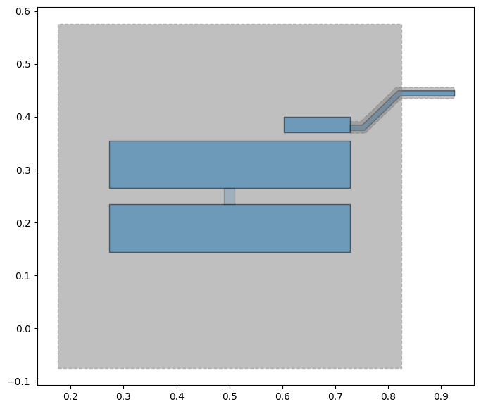
What just happened?
In a few lines you:
Created a quantum chip design canvas (
DesignPlanar)Placed a superconducting transmon qubit on it (
TransmonPocket)Rendered it to a matplotlib figure — no Qt, no GUI, no extra setup
The rest of this tutorial unpacks what each step means and how to control every detail. Skip ahead to 1.2 Your First Chip if you want to keep building immediately.
The Quantum Metal design flow
Designing a superconducting chip in Quantum Metal is a four-step loop:
Pick a design canvas (
DesignPlanar,DesignFlipChip, …).Place QComponents — transmons, couplers, routes, terminations.
Render to your backend of choice: GDS for fabrication, HFSS/Q3D or open FEM (gmsh + Elmer / AWS Palace) for simulation.
Analyse — Hamiltonian, capacitance, eigenmodes, EPR.
This tutorial focuses on the first two steps and shows both the inline matplotlib view (qm.view) and the desktop GUI (MetalGUI) — qm.gui(design) picks the right one automatically.
Step 1 → 4: from design to fab
flowchart LR
    A[<b>1. Design</b><br/><code>DesignPlanar()</code><br/>Pick a chip canvas]
    B[<b>2. Place QComponents</b><br/>Transmons, couplers,<br/>routes, terminations]
    C[<b>3. Render</b><br/>GDS, HFSS / Q3D,<br/>gmsh + Elmer / Palace]
    D[<b>4. Analyse</b><br/>Hamiltonian, capacitance,<br/>eigenmodes, EPR]
    A --> B --> C --> D
    D -. iterate .-> B
    classDef pri fill:#6929C4,stroke:#3D1773,color:#fff
    classDef sec fill:#e8defc,stroke:#6929C4,color:#1a1a1a
    class A,C pri
    class B,D sec
This tutorial focuses on steps 1 and 2 — creating a design and adding components. Tutorial 1.3 covers step 3 (export to GDS); the 4-Analysis tutorials cover step 4.
How to follow along
You can run Quantum Metal in three ways:
Jupyter / Colab / Binder — interactive, fastest for exploration. The Colab badge at the top of this notebook installs the lite (no-Qt) wheel in seconds.
Plain Python scripts — for reproducible CI / batch runs.
Desktop ``MetalGUI`` — the Qt-based interactive editor (
pip install 'quantum-metal[gui]').
The same Python API drives all three. qm.gui(design) returns the desktop GUI when Qt is available, an inline viewer otherwise — your tutorial code is identical in both paths.
What lives inside a QDesign
flowchart TB
    subgraph design[QDesign — the chip canvas]
        components[design.components<br/><i>Dict of QComponent instances</i>]
        variables[design.variables<br/><i>shared option values</i>]
        chips[design.chips<br/><i>chip stack + materials</i>]
        qg[design.qgeometry<br/><i>per-component shapely tables</i>]
    end

    qc[QComponent subclasses<br/>TransmonPocket, RouteMeander, ...] --> components
    components -. options -.-> qg
    components -. pins -.-> components

    qg --> rend[QRenderer]
    rend --> gds[GDS file]
    rend --> hfss[HFSS / Q3D project]
    rend --> fem[gmsh + Elmer / Palace]

    classDef inner fill:#f4f1fb,stroke:#6929C4,color:#1a1a1a
    classDef outer fill:#6929C4,stroke:#3D1773,color:#fff
    class components,variables,chips,qg inner
    class qc,rend outer
Every QComponent you instantiate registers itself on design.components. Calling gui.rebuild() (or design.rebuild()) re-runs each component’s make() against current option values and refreshes design.qgeometry. Renderers consume that geometry to produce GDS files, HFSS/Q3D projects, or open-FEM meshes.
Building blocks
Quantum Metal organises a chip around a few abstractions:
``QComponent`` — a physical piece (transmon, CPW, launchpad). You instantiate subclasses, not
QComponentitself.``QDesign`` — the chip canvas; holds components, variables, and chip geometry.
``QRenderer`` — converts the design to a target format (GDS, HFSS, Q3D, gmsh, Elmer, …).
``QGeometry`` — the per-component shapely shapes (polygons, paths, junctions).
Import Quantum Metal
[2]:
import qiskit_metal as metal
from qiskit_metal import designs, draw
from qiskit_metal import open_docs

%metal_heading Welcome to Qiskit Metal!
Welcome to Qiskit Metal!
If you see the welcome banner, the install is healthy. Onward.
Create a design
Every chip starts from a QDesign. DesignPlanar is the simplest — a single planar chip.
[3]:
design = designs.DesignPlanar()
Re-running cells safely
While iterating you’ll re-instantiate components a lot. Tell the design to overwrite previous versions silently:
[4]:
design.overwrite_enabled = True
[5]:
%metal_heading Hello Quantum World!
Hello Quantum World!
Chip dimensions
Each design has a default chip called main. Inspect or resize it via design.chips.main.size.
[6]:
# We can also check all of the chip properties to see if we want to change the size or any other parameter.
# By default the name of chip is "main".
design.chips.main
[6]:
{'material': 'silicon',
 'layer_start': '0',
 'layer_end': '2048',
 'size': {'center_x': '0.0mm',
  'center_y': '0.0mm',
  'center_z': '0.0mm',
  'size_x': '9mm',
  'size_y': '6mm',
  'size_z': '-750um',
  'sample_holder_top': '890um',
  'sample_holder_bottom': '1650um'}}
Update any dimension by assigning to the dict; gui.rebuild() propagates the change.
[7]:
design.chips.main.size.size_x = "11mm"
design.chips.main.size.size_y = "9mm"
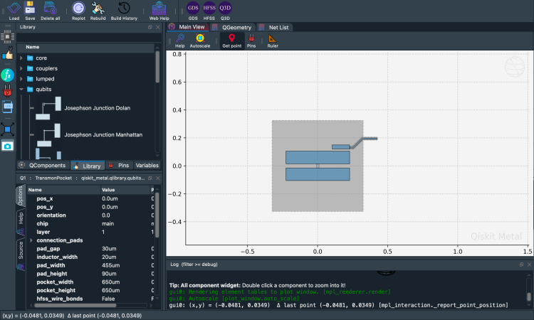
Launching the viewer
qm.gui(design) returns either the desktop MetalGUI (Qt) or MetalGUIHeadless (inline matplotlib). The tutorial-facing API — gui.rebuild(), gui.autoscale(), gui.screenshot(), gui.edit_component(...) — is the same in both.
[8]:
gui = qm.gui(design)
Either a Qt window opens or an inline figure renders below. Either way you’re ready to place components.
Place your first qubit
Time to add a TransmonPocket — a ready-made transmon from qiskit_metal.qlibrary.qubits.
[9]:
# Select a QComponent to create (The QComponent is a python class named `TransmonPocket`)
from qiskit_metal.qlibrary.qubits.transmon_pocket import TransmonPocket


q1 = TransmonPocket(
    design, "Q1", options=dict(connection_pads=dict(a=dict()))
)  # Create a new Transmon Pocket object with name 'Q1'
gui.rebuild()  # rebuild the design and plot

gui.edit_component("Q1")  # set Q1 as the editable component
gui.autoscale()  # resize GUI to see QComponent
Print the component object to inspect its name, type, and resolved options:
[10]:
q1 # print Q1 information
[10]:
name:    Q1
class:   TransmonPocket
options:
  'pos_x'             : '0.0um',
  'pos_y'             : '0.0um',
  'orientation'       : '0.0',
  'chip'              : 'main',
  'layer'             : '1',
  'connection_pads'   : {
       'a'                 : {
            'pad_gap'           : '15um',
            'pad_width'         : '125um',
            'pad_height'        : '30um',
            'pad_cpw_shift'     : '5um',
            'pad_cpw_extent'    : '25um',
            'cpw_width'         : 'cpw_width',
            'cpw_gap'           : 'cpw_gap',
            'cpw_extend'        : '100um',
            'pocket_extent'     : '5um',
            'pocket_rise'       : '65um',
            'loc_W'             : '+1',
            'loc_H'             : '+1',
                             },
                        },
  'pad_gap'           : '30um',
  'inductor_width'    : '20um',
  'pad_width'         : '455um',
  'pad_height'        : '90um',
  'pocket_width'      : '650um',
  'pocket_height'     : '650um',
  'hfss_wire_bonds'   : False,
  'q3d_wire_bonds'    : False,
  'aedt_q3d_wire_bonds': False,
  'aedt_hfss_wire_bonds': False,
  'hfss_inductance'   : '10nH',
  'hfss_capacitance'  : 0,
  'hfss_resistance'   : 0,
  'hfss_mesh_kw_jj'   : 7e-06,
  'q3d_inductance'    : '10nH',
  'q3d_capacitance'   : 0,
  'q3d_resistance'    : 0,
  'q3d_mesh_kw_jj'    : 7e-06,
  'gds_cell_name'     : 'my_other_junction',
  'aedt_q3d_inductance': 1e-08,
  'aedt_q3d_capacitance': 0,
  'aedt_hfss_inductance': 1e-08,
  'aedt_hfss_capacitance': 0,
module:  qiskit_metal.qlibrary.qubits.transmon_pocket
id:      1
[ ]:
gui.screenshot() # screenshot of the design in GUI
Default options
Each QComponent ships with a default_options dict (pad sizes, position, layer, etc.). Quantum Metal parses the strings into numbers during make(). You can change options through the GUI or the Python API — they call the same setters.
[11]:
%metal_print How do I edit options? API or GUI
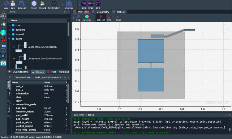
Updating components
Mutate q1.options.<field> and call gui.rebuild(). The GUI re-renders the geometry from the new options.
[12]:
# Change options
q1.options.pos_x = "0.5 mm"
q1.options.pos_y = "0.25 mm"
q1.options.pad_height = "225 um"
q1.options.pad_width = "250 um"
q1.options.pad_gap = "50 um"
Rebuilding
gui.rebuild() re-runs every component’s make() against current option values and updates the displayed geometry. Call it after any option change.
[13]:
gui.rebuild()  # Update the component geometry, since we changed the options

# Get a list of all the qcomponents in QDesign and then zoom on them.
all_component_names = design.components.keys()

gui.zoom_on_components(all_component_names)

# An alternate way to view within GUI. If want to try it, remove the "#" from the beginning of line.
# gui.autoscale() #resize GUI
[18]:
gui.screenshot() # screenshot of the design in GUI
Closing the viewer
[ ]:
# gui.main_window.close()
Next steps
Tutorial 1.1 Quick start walks through the same flow in more depth, including variables, pin-to-pin connections with RouteMeander, and a full 4-qubit chip. For an entirely Qt-free walk, see 1.1 Quick start.
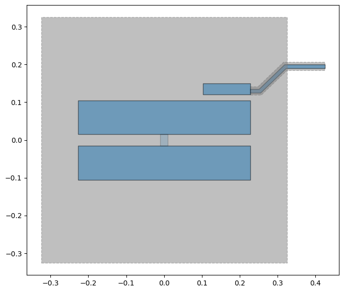
[18]:
%matplotlib inline
[19]:
fig = qm.view(design)
fig  # inline-display in Jupyter; fig.savefig("...") to write to file
[19]:
For more information, review the Introduction to Quantum Computing and Quantum Hardware lectures below
|
Lecture Video | Lecture Notes | Lab |
|
Lecture Video | Lecture Notes | Lab |
|
Lecture Video | Lecture Notes | Lab |
|
Lecture Video | Lecture Notes | Lab |
|
Lecture Video | Lecture Notes | Lab |
|
Lecture Video | Lecture Notes | Lab |