Note
This page was generated from tut/4-Analysis/4.23-Impedance-and-scattering-Z-S-Y-matrices.ipynb.
4.23 Sweeps - Impedance, scattering and admittance (Z S Y) matrices
Prerequisite
You need to have a working local installation of Ansys
1. Perform the necessary imports and create a QDesign in Metal first.
[2]:
import qiskit_metal as metal
from qiskit_metal import designs, draw
from qiskit_metal import MetalGUI, Dict, Headings
import pyEPR as epr
from qiskit_metal.analyses.simulation import ScatteringImpedanceSim
Create the design in Metal
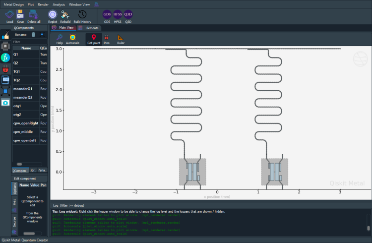
Set up a design of a given dimension. Create a design by specifying the chip size and open Metal GUI. Dimensions will be respected in the design rendering. Note the chip design is centered at origin (0,0).
[3]:
design = designs.DesignPlanar({}, True)
design.chips.main.size["size_x"] = "2mm"
design.chips.main.size["size_y"] = "2mm"

gui = MetalGUI(design)

# Perform the necessary imports.
from qiskit_metal.qlibrary.couplers.coupled_line_tee import CoupledLineTee
from qiskit_metal.qlibrary.tlines.meandered import RouteMeander
from qiskit_metal.qlibrary.qubits.transmon_pocket import TransmonPocket
from qiskit_metal.qlibrary.tlines.straight_path import RouteStraight
from qiskit_metal.qlibrary.terminations.open_to_ground import OpenToGround
[4]:
# To create plots after geting solution data.
import matplotlib.pyplot as plt
import numpy as np
[5]:
# Add 2 transmons to the design.
options = dict(
    # Some options we want to modify from the deafults
    # (see below for defaults)
    pad_width="425 um",
    pocket_height="650um",
    # Adding 4 connectors (see below for defaults)
    connection_pads=dict(
        a=dict(loc_W=+1, loc_H=+1),
        b=dict(loc_W=-1, loc_H=+1, pad_height="30um"),
        c=dict(loc_W=+1, loc_H=-1, pad_width="200um"),
        d=dict(loc_W=-1, loc_H=-1, pad_height="50um"),
    ),
)

## Create 2 transmons
q1 = TransmonPocket(
    design, "Q1", options=dict(pos_x="+1.4mm", pos_y="0mm", orientation="90", **options)
)
q2 = TransmonPocket(
    design, "Q2", options=dict(pos_x="-0.6mm", pos_y="0mm", orientation="90", **options)
)

gui.rebuild()
gui.autoscale()
[6]:
# Add 2 hangers consisting of capacitively coupled transmission lines.
TQ1 = CoupledLineTee(
    design,
    "TQ1",
    options=dict(
        pos_x="1mm", pos_y="3mm", coupling_length="500um", coupling_space="1um"
    ),
)
TQ2 = CoupledLineTee(
    design,
    "TQ2",
    options=dict(
        pos_x="-1mm", pos_y="3mm", coupling_length="500um", coupling_space="1um"
    ),
)

gui.rebuild()
gui.autoscale()
[7]:
# Add 2 meandered CPWs connecting the transmons to the hangers.
ops = dict(fillet="90um")
design.overwrite_enabled = True

options1 = Dict(
    total_length="8mm",
    hfss_wire_bonds=True,
    pin_inputs=Dict(
        start_pin=Dict(component="TQ1", pin="second_end"),
        end_pin=Dict(component="Q1", pin="a"),
    ),
    lead=Dict(start_straight="0.1mm"),
    **ops,
)

options2 = Dict(
    total_length="9mm",
    hfss_wire_bonds=True,
    pin_inputs=Dict(
        start_pin=Dict(component="TQ2", pin="second_end"),
        end_pin=Dict(component="Q2", pin="a"),
    ),
    lead=Dict(start_straight="0.1mm"),
    **ops,
)

meanderQ1 = RouteMeander(design, "meanderQ1", options=options1)
meanderQ2 = RouteMeander(design, "meanderQ2", options=options2)

gui.rebuild()
gui.autoscale()
[8]:
# Add 2 open to grounds at the ends of the horizontal CPW.
otg1 = OpenToGround(design, "otg1", options=dict(pos_x="3mm", pos_y="3mm"))
otg2 = OpenToGround(
    design, "otg2", options=dict(pos_x="-3mm", pos_y="3mm", orientation="180")
)

gui.rebuild()
gui.autoscale()

# Add 3 straight CPWs that comprise the long horizontal CPW.

ops_oR = Dict(
    hfss_wire_bonds=True,
    pin_inputs=Dict(
        start_pin=Dict(component="TQ1", pin="prime_end"),
        end_pin=Dict(component="otg1", pin="open"),
    ),
)
ops_mid = Dict(
    hfss_wire_bonds=True,
    pin_inputs=Dict(
        start_pin=Dict(component="TQ1", pin="prime_start"),
        end_pin=Dict(component="TQ2", pin="prime_end"),
    ),
)
ops_oL = Dict(
    hfss_wire_bonds=True,
    pin_inputs=Dict(
        start_pin=Dict(component="TQ2", pin="prime_start"),
        end_pin=Dict(component="otg2", pin="open"),
    ),
)

cpw_openRight = RouteStraight(design, "cpw_openRight", options=ops_oR)
cpw_middle = RouteStraight(design, "cpw_middle", options=ops_mid)
cpw_openLeft = RouteStraight(design, "cpw_openLeft", options=ops_oL)

gui.rebuild()
gui.autoscale()
[9]:
gui.screenshot()
2. Render the qubit from Metal into the HangingResonators design in Ansys. ScatteringImpedanceSim will open the simulation software. Then will connect, activate the design, add a setup.
Review and update the setup. For driven modal you will need to define not only the simulation convergence parameters, but also the frequency sweep.
[10]:
em1 = ScatteringImpedanceSim(design, "hfss")
Customizable parameters and default values for HFSS (driven modal):
freq_ghz=5 (simulation frequency)
name="Setup" (setup name)
max_delta_s=0.1 (absolute value of maximum difference in scattering parameter S)
max_passes=10 (maximum number of passes)
min_passes=1 (minimum number of passes)
min_converged=1 (minimum number of converged passes)
pct_refinement=30 (percent refinement)
basis_order=1 (basis order)
vars (global variables to set in the renderer)
sweep_setup (all the parameters of the sweep)
name="Sweep" (name of sweep)
start_ghz=2.0 (starting frequency)
stop_ghz=8.0 (stopping frequency)
count=101 (total number of frequencies)
step_ghz=None (frequency step size)
type="Fast" (type of sweep)
save_fields=False (whether or not to save fields)
[11]:
# To view the values for defaults.
em1.setup
[11]:
{'name': 'Setup',
 'reuse_selected_design': True,
 'reuse_setup': True,
 'freq_ghz': 5,
 'max_delta_s': 0.1,
 'max_passes': 10,
 'min_passes': 1,
 'min_converged': 1,
 'pct_refinement': 30,
 'basis_order': 1,
 'vars': {'Lj': '10 nH', 'Cj': '0 fF'},
 'sweep_setup': {'name': 'Sweep',
  'start_ghz': 2.0,
  'stop_ghz': 8.0,
  'count': 101,
  'step_ghz': None,
  'type': 'Fast',
  'save_fields': False}}
[12]:
em1.setup.name = "Sweep_DrivenModal_setup"
em1.setup.freq_ghz = 6.0
em1.setup.max_delta_s = 0.05
em1.setup.max_passes = 12
em1.setup.min_passes = 2
Add a frequency sweep to a driven modal setup. From QHFSSRenderer.add_sweep doc_strings. Please go to doc_strings to get the latest information.
Args: setup_name (str, optional): Name of driven modal simulation Sweep. Defaults to “Setup”. start_ghz (float, optional): Starting frequency of sweep in GHz. Defaults to 2.0. stop_ghz (float, optional): Ending frequency of sweep in GHz. Defaults to 8.0. count (int, optional): Total number of frequencies. Defaults to 101. step_ghz (float, optional): Difference between adjacent frequencies. Defaults to None. name (str, optional): Name of sweep. Defaults to “Sweep”. type (str, optional): Type of sweep. Defaults to “Fast”. save_fields (bool, optional): Whether or not to save fields. Defaults to False.
[13]:
# To view the values for defaults.
em1.setup.sweep_setup
[13]:
{'name': 'Sweep',
 'start_ghz': 2.0,
 'stop_ghz': 8.0,
 'count': 101,
 'step_ghz': None,
 'type': 'Fast',
 'save_fields': False}
[14]:
em1.setup.sweep_setup.name = "Sweep_options__dm_sweep"
em1.setup.sweep_setup.start_ghz = 4.0
em1.setup.sweep_setup.stop_ghz = 9.0
em1.setup.sweep_setup.count = 5001
em1.setup.sweep_setup.type = "Interpolating"


em1.setup
[14]:
{'name': 'Sweep_DrivenModal_setup',
 'reuse_selected_design': True,
 'reuse_setup': True,
 'freq_ghz': 6.0,
 'max_delta_s': 0.05,
 'max_passes': 12,
 'min_passes': 2,
 'min_converged': 1,
 'pct_refinement': 30,
 'basis_order': 1,
 'vars': {'Lj': '10 nH', 'Cj': '0 fF'},
 'sweep_setup': {'name': 'Sweep_options__dm_sweep',
  'start_ghz': 4.0,
  'stop_ghz': 9.0,
  'count': 5001,
  'step_ghz': None,
  'type': 'Interpolating',
  'save_fields': False}}
[15]:
# Set the buffer width at the edge of the design to be 0.5 mm
# in both directions.
em1.setup.renderer.options["x_buffer_width_mm"] = 0.5
em1.setup.renderer.options["y_buffer_width_mm"] = 0.5
[16]:
#     qcomp_name (str): A component that contains the option to be swept.
#     option_name (str): The option within qcomp_name to sweep.
#     option_sweep (list): Each entry in the list is a value for
#                 option_name.
#     qcomp_render (list): The component to render to simulation.
#     open_terminations (list): Identify which kind of pins. Follow the
#                 details from renderer QQ3DRenderer.render_design, or
#                 QHFSSRenderer.render_design.
#     port_list (list): List of tuples of jj's that shouldn't
#                     be rendered.  Follow details from
#                     renderer in QHFSSRenderer.render_design.
#     jj_to_port (list): List of junctions (qcomp, qgeometry_name,
#                         impedance, draw_ind) to render as lumped ports
#                         or as lumped port in parallel with a sheet
#                         inductance.    Follow details from renderer
#                         in QHFSSRenderer.render_design.
#     ignored_jjs (Union[list,None]): This is not used by all renderers,
#                  just hfss.
#     design_name(str): Name of design (workspace) to use in project.
#     box_plus_buffer(bool): Render the entire chip or create a
#                 box_plus_buffer around the components which are rendered.
[17]:
design_name = "Sweep_DrivenModal"
qcomp_render = []  # Means to render everything in qgeometry table.
open_terminations = []

# Here, pin cpw_openRight_end and cpw_openLeft_end are converted into lumped ports,
#           each with an impedance of 50 Ohms. <br>
port_list = [("cpw_openRight", "end", 50), ("cpw_openLeft", "end", 50)]
jj_to_port = [("Q1", "rect_jj", 50, False)]
# Neither of the junctions in Q1 or Q2 are rendered.
ignored_jjs = [("Q2", "rect_jj")]
box_plus_buffer = True
[18]:
# Note: The method will connect to  Ansys simulation, activate_drivenmodal_design(), add_drivenmodal_setup().

all_sweeps, return_code = em1.run_sweep(
    meanderQ1.name,
    "total_length",
    ["9mm", "10mm", "11mm"],
    qcomp_render,
    open_terminations,
    design_name=design_name,
    port_list=port_list,
    jj_to_port=jj_to_port,
    ignored_jjs=ignored_jjs,
    box_plus_buffer=box_plus_buffer,
)
INFO 08:57AM [connect_project]: Connecting to Ansys Desktop API...
INFO 08:57AM [load_ansys_project]:      Opened Ansys App
INFO 08:57AM [load_ansys_project]:      Opened Ansys Desktop v2020.2.0
INFO 08:57AM [load_ansys_project]:      Opened Ansys Project
        Folder:    C:/Ansoft/
        Project:   Project24
INFO 08:57AM [connect_design]: No active design found (or error getting active design).
INFO 08:57AM [connect]:          Connected to project "Project24". No design detected
INFO 08:57AM [connect_design]:  Opened active design
        Design:    Sweep_DrivenModal_hfss [Solution type: DrivenModal]
WARNING 08:57AM [connect_setup]:        No design setup detected.
WARNING 08:57AM [connect_setup]:        Creating drivenmodal default setup.
INFO 08:57AM [get_setup]:       Opened setup `Setup`  (<class 'pyEPR.ansys.HfssDMSetup'>)
INFO 08:58AM [get_setup]:       Opened setup `Sweep_DrivenModal_setup`  (<class 'pyEPR.ansys.HfssDMSetup'>)
INFO 08:58AM [get_setup]:       Opened setup `Sweep_DrivenModal_setup`  (<class 'pyEPR.ansys.HfssDMSetup'>)
INFO 08:58AM [analyze]: Analyzing setup Sweep_DrivenModal_setup : Sweep_options__dm_sweep
INFO 09:01AM [connect_design]:  Opened active design
        Design:    Sweep_DrivenModal_hfss [Solution type: DrivenModal]
INFO 09:02AM [get_setup]:       Opened setup `Sweep_DrivenModal_setup`  (<class 'pyEPR.ansys.HfssDMSetup'>)
INFO 09:02AM [get_setup]:       Opened setup `Sweep_DrivenModal_setup`  (<class 'pyEPR.ansys.HfssDMSetup'>)
INFO 09:02AM [analyze]: Analyzing setup Sweep_DrivenModal_setup : Sweep_options__dm_sweep
INFO 09:07AM [connect_design]:  Opened active design
        Design:    Sweep_DrivenModal_hfss [Solution type: DrivenModal]
INFO 09:07AM [get_setup]:       Opened setup `Sweep_DrivenModal_setup`  (<class 'pyEPR.ansys.HfssDMSetup'>)
INFO 09:07AM [get_setup]:       Opened setup `Sweep_DrivenModal_setup`  (<class 'pyEPR.ansys.HfssDMSetup'>)
INFO 09:07AM [analyze]: Analyzing setup Sweep_DrivenModal_setup : Sweep_options__dm_sweep
#Note: Sweep again using the arguments from previous run.
all_sweeps_6_7_8, return_code = em1.run_sweep(meanderQ1.name,
                                        'total_length',
                                        ['6.5mm', '7.5mm', '8.5mm']
                                       )
[19]:
if return_code == 0:
    # Each key corresponds to list passed to ['9mm', '8mm', '7mm']
    print(all_sweeps.keys())

    # Each key corresponds to list passed to ['6mm', '5mm', '4mm']
    # print(all_sweeps_6_7_8.keys())
else:
    print("Check warning messages to see why all_sweeps is non-zero.")
dict_keys(['9mm', '10mm', '11mm'])
[20]:
all_sweeps["9mm"].keys()
[20]:
dict_keys(['option_name', 'variables'])
[21]:
all_sweeps["9mm"]["variables"]
[21]:
{'sim_setup_name': 'Sweep_DrivenModal_setup',
 'sweep_name': 'Sweep_options__dm_sweep'}
[22]:
all_sweeps["9mm"]["option_name"]
[22]:
'total_length'
[23]:
print(f"""
project_name = {em1.renderer.pinfo.project_name}
design_name  = {em1.renderer.pinfo.design_name}
setup_name   = {em1.renderer.pinfo.setup_name}
""")
project_name = Project24
design_name  = Sweep_DrivenModal_hfss
setup_name   = Sweep_DrivenModal_setup
Note: Results storage is currently being updated to be fully functional with the sweep functionality.
[24]:
em1.get_impedance() # default: ['Z11', 'Z21']
[24]:
(                        Z11                   Z21
 4.000  -0.000000-11.896548j   0.000000+44.291514j
 4.001   0.000001-11.881640j   0.00000+044.287660j
 4.002   0.000001-11.866735j   0.000000+44.283811j
 4.003   0.000002-11.851833j   0.000000+44.279968j
 4.004   0.000002-11.836933j   0.000000+44.276131j
 ...                     ...                   ...
 8.996  0.000429+233.181228j  0.000398+237.847267j
 8.997  0.000331+233.625173j  0.000307+238.283674j
 8.998  0.000228+234.070780j  0.000211+238.721763j
 8.999  0.000117+234.518060j  0.000109+239.161547j
 9.000 -0.000000+234.967023j -0.000000+239.603035j

 [5001 rows x 2 columns],
 <Figure size 3000x1800 with 2 Axes>)
[25]:
em1.get_admittance() # default: ['Y11', 'Y21']
[25]:
(                      Y11                 Y21
 4.000  0.000000-0.006633j -0.000000-0.024359j
 4.001  0.000000-0.006625j  0.000000-0.024357j
 4.002  0.000000-0.006617j  0.000000-0.024355j
 4.003  0.000000-0.006609j  0.000000-0.024352j
 4.004  0.000000-0.006600j  0.000000-0.024350j
 ...                   ...                 ...
 8.996 -0.000000+0.086442j  0.000000-0.088951j
 8.997 -0.000000+0.086555j  0.000000-0.089060j
 8.998 -0.000000+0.086669j  0.000000-0.089169j
 8.999 -0.000000+0.086783j  0.000000-0.089279j
 9.000  0.000000+0.086898j -0.000000-0.089390j

 [5001 rows x 2 columns],
 <Figure size 3000x1800 with 2 Axes>)
[26]:
em1.get_scattering(["S11", "S21", "S31"]) ## default: ['S11', 'S21', 'S22']
[26]:
(                      S11                 S21                 S31
 4.000 -0.147086-0.038897j -0.264193+0.952394j  0.000055+0.000028j
 4.001 -0.147108-0.038852j -0.263887+0.952478j  0.000055+0.000028j
 4.002 -0.147130-0.038806j -0.263581+0.952561j  0.000055+0.000028j
 4.003 -0.147152-0.038761j -0.263275+0.952644j  0.000055+0.000028j
 4.004 -0.147174-0.038715j -0.262969+0.952727j  0.000055+0.000028j
 ...                   ...                 ...                 ...
 8.996  0.005780-0.006204j  0.976020+0.217516j -0.000039+0.000050j
 8.997  0.005783-0.006260j  0.976093+0.217185j -0.000039+0.000050j
 8.998  0.005786-0.006317j  0.976166+0.216855j -0.000039+0.000050j
 8.999  0.005790-0.006373j  0.976239+0.216524j -0.000039+0.000050j
 9.000  0.005793-0.006430j  0.976312+0.216192j -0.000039+0.000050j

 [5001 rows x 3 columns],
 <Figure size 3000x1800 with 2 Axes>)
[27]:
dataframe_scattering = em1.get_scattering(["S11", "S21", "S31"])
df_s = dataframe_scattering[0]
[28]:
s11 = df_s["S11"]
s11

s21 = df_s["S21"]
s21

s31 = df_s["S31"]
s31
[28]:
4.000    0.000055+0.000028j
4.001    0.000055+0.000028j
4.002    0.000055+0.000028j
4.003    0.000055+0.000028j
4.004    0.000055+0.000028j
                ...
8.996   -0.000039+0.000050j
8.997   -0.000039+0.000050j
8.998   -0.000039+0.000050j
8.999   -0.000039+0.000050j
9.000   -0.000039+0.000050j
Name: S31, Length: 5001, dtype: complex128
[29]:
dataframe_scattering[0]["20_log_of_mag_S11"] = 20 * np.log10(np.absolute(s11))
dataframe_scattering[0]["20_log_of_mag_S21"] = 20 * np.log10(np.absolute(s21))
dataframe_scattering[0]["20_log_of_mag_S31"] = 20 * np.log10(np.absolute(s31))
dataframe_scattering[0]
[29]:
| S11 | S21 | S31 | 20_log_of_mag_S11 | 20_log_of_mag_S21 | 20_log_of_mag_S31 | |
|---|---|---|---|---|---|---|
| 4.000 | -0.147086-0.038897j | -0.264193+0.952394j | 0.000055+0.000028j | -16.355031 | -0.101708 | -84.181500 |
| 4.001 | -0.147108-0.038852j | -0.263887+0.952478j | 0.000055+0.000028j | -16.354476 | -0.101722 | -84.199503 |
| 4.002 | -0.147130-0.038806j | -0.263581+0.952561j | 0.000055+0.000028j | -16.353923 | -0.101735 | -84.217446 |
| 4.003 | -0.147152-0.038761j | -0.263275+0.952644j | 0.000055+0.000028j | -16.353370 | -0.101748 | -84.235327 |
| 4.004 | -0.147174-0.038715j | -0.262969+0.952727j | 0.000055+0.000028j | -16.352819 | -0.101761 | -84.253149 |
| ... | ... | ... | ... | ... | ... | ... |
| 8.996 | 0.005780-0.006204j | 0.976020+0.217516j | -0.000039+0.000050j | -41.433315 | -0.000314 | -83.990805 |
| 8.997 | 0.005783-0.006260j | 0.976093+0.217185j | -0.000039+0.000050j | -41.388457 | -0.000317 | -83.990549 |
| 8.998 | 0.005786-0.006317j | 0.976166+0.216855j | -0.000039+0.000050j | -41.343861 | -0.000319 | -83.990273 |
| 8.999 | 0.005790-0.006373j | 0.976239+0.216524j | -0.000039+0.000050j | -41.299529 | -0.000322 | -83.989977 |
| 9.000 | 0.005793-0.006430j | 0.976312+0.216192j | -0.000039+0.000050j | -41.255465 | -0.000325 | -83.989660 |
5001 rows × 6 columns
[30]:
# Reference to current axis.
magnitude = plt.figure("Magnitude S11, S21, and S31")
plt.clf()
axis = plt.gca()  # Get current axis.
dataframe_scattering[0].plot(kind="line", y="20_log_of_mag_S11", color="green", ax=axis)
dataframe_scattering[0].plot(kind="line", y="20_log_of_mag_S21", color="blue", ax=axis)
dataframe_scattering[0].plot(kind="line", y="20_log_of_mag_S31", color="red", ax=axis)
plt.title("S-Parameter Magnitude")
plt.xlabel("frequency [GHZ]")
plt.ylabel("|S11|,|S21|,|S31| [dB]")
magnitude.show()
[31]:
# Data is shown as degrees.
# However, if you want radians, change value of deg to false, deg=False.
dataframe_scattering[0]["degrees_S11"] = np.angle(s11, deg=True)
dataframe_scattering[0]["degrees_S21"] = np.angle(s21, deg=True)
dataframe_scattering[0]["degrees_S31"] = np.angle(s31, deg=True)
dataframe_scattering[0]
[31]:
| S11 | S21 | S31 | 20_log_of_mag_S11 | 20_log_of_mag_S21 | 20_log_of_mag_S31 | degrees_S11 | degrees_S21 | degrees_S31 | |
|---|---|---|---|---|---|---|---|---|---|
| 4.000 | -0.147086-0.038897j | -0.264193+0.952394j | 0.000055+0.000028j | -16.355031 | -0.101708 | -84.181500 | -165.187158 | 105.503950 | 27.027756 |
| 4.001 | -0.147108-0.038852j | -0.263887+0.952478j | 0.000055+0.000028j | -16.354476 | -0.101722 | -84.199503 | -165.205819 | 105.485570 | 27.012771 |
| 4.002 | -0.147130-0.038806j | -0.263581+0.952561j | 0.000055+0.000028j | -16.353923 | -0.101735 | -84.217446 | -165.224480 | 105.467191 | 26.997785 |
| 4.003 | -0.147152-0.038761j | -0.263275+0.952644j | 0.000055+0.000028j | -16.353370 | -0.101748 | -84.235327 | -165.243140 | 105.448812 | 26.982800 |
| 4.004 | -0.147174-0.038715j | -0.262969+0.952727j | 0.000055+0.000028j | -16.352819 | -0.101761 | -84.253149 | -165.261801 | 105.430433 | 26.967815 |
| ... | ... | ... | ... | ... | ... | ... | ... | ... | ... |
| 8.996 | 0.005780-0.006204j | 0.976020+0.217516j | -0.000039+0.000050j | -41.433315 | -0.000314 | -83.990805 | -47.027252 | 12.563626 | 128.377355 |
| 8.997 | 0.005783-0.006260j | 0.976093+0.217185j | -0.000039+0.000050j | -41.388457 | -0.000317 | -83.990549 | -47.269117 | 12.544227 | 128.350189 |
| 8.998 | 0.005786-0.006317j | 0.976166+0.216855j | -0.000039+0.000050j | -41.343861 | -0.000319 | -83.990273 | -47.509012 | 12.524818 | 128.322852 |
| 8.999 | 0.005790-0.006373j | 0.976239+0.216524j | -0.000039+0.000050j | -41.299529 | -0.000322 | -83.989977 | -47.746983 | 12.505400 | 128.295342 |
| 9.000 | 0.005793-0.006430j | 0.976312+0.216192j | -0.000039+0.000050j | -41.255465 | -0.000325 | -83.989660 | -47.983072 | 12.485973 | 128.267657 |
5001 rows × 9 columns
[32]:
# Reference to current axis.
phase = plt.figure("Phase of S11 and S21")
plt.clf()
axis = plt.gca()  # Get current axis.
dataframe_scattering[0].plot(kind="line", y="degrees_S11", color="green", ax=axis)
dataframe_scattering[0].plot(kind="line", y="degrees_S21", color="blue", ax=axis)
dataframe_scattering[0].plot(kind="line", y="degrees_S31", color="red", ax=axis)
plt.title("S-Parameter Phase")
plt.xlabel("frequency [GHZ]")
plt.ylabel("<S11, <S21, <S31 [degrees]")
phase.show()
[33]:
em1.close()
[34]:
# Uncomment next line if you would like to close the gui
# gui.main_window.close()
For more information, review the Introduction to Quantum Computing and Quantum Hardware lectures below
|
Lecture Video | Lecture Notes | Lab |
|
Lecture Video | Lecture Notes | Lab |
|
Lecture Video | Lecture Notes | Lab |
|
Lecture Video | Lecture Notes | Lab |
|
Lecture Video | Lecture Notes | Lab |
|
Lecture Video | Lecture Notes | Lab |