Note
This page was generated from tut/1-Overview/1.1-Bird’s-eye-view-of-Qiskit-Metal.ipynb.
1.1 Bird’s eye view of Quantum Metal (Formerly: Qiskit Metal)
💡 Using this tutorial without the Qt GUI
This tutorial uses the desktop
MetalGUIand includes screenshots of what it looks like. The Qt GUI is optional — the full Quantum Metal API works without it.To follow along on Colab, Binder, JupyterHub, or any headless environment, replace any
gui.rebuild()orgui.screenshot()call withqm.view(design)to render the design inline as a matplotlib figure.See 1.4 Headless quick view for a complete runnable walkthrough.
[ ]:
# Three lines to your first superconducting qubit
import qiskit_metal as qm
from qiskit_metal import designs
from qiskit_metal.qlibrary.qubits.transmon_pocket import TransmonPocket

design = designs.DesignPlanar()
q1 = TransmonPocket(
    design,
    "Q1",
    options=dict(
        pos_x="0.5mm",
        pos_y="0.25mm",
        connection_pads=dict(a=dict(loc_W=+1, loc_H=+1)),
    ),
)
fig = qm.view(design)
fig
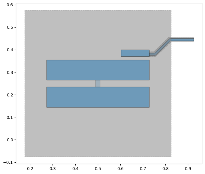
What just happened?
In a few lines you:
Created a quantum chip design canvas (
DesignPlanar)Placed a superconducting transmon qubit on it (
TransmonPocket)Rendered it to a matplotlib figure — no Qt, no GUI, no extra setup
The rest of this tutorial unpacks what each step means and how to control every detail. Skip ahead to 1.2 Your First Chip if you want to keep building immediately.
🌟 The Qiskit Metal Design Flow — Your 4-Step Adventure 🌟
Let’s walk through the four stages you’ll use again and again:
1. Pick a Design Class 🏗️
2. Add & Customize Components 🎨
3. Render → Simulate → Analyze 🔍
Once your design looks good, it’s time to explore how it behaves.
Current Rendering & Simulation Options:
Ansys Integration
HFSS Renderer — for high-frequency simulations (eigenmode, modal, terminal)
EPR Analysis → computes energy participation ratios
Q3D Renderer — extracts layout-based equivalent circuit parameters (e.g., capacitances)
LOM Analysis → uses Q3D capacitances to evaluate transmon parameters
This is the “science happens here” step. 🔬✨
4. Render for Fabrication 🏭
When you’re ready to turn your design into something real:
GDS Renderer Output clean, fabrication-ready GDSII files that you can send to your foundry.
🎯 Visual Summary
All of these steps come together in the diagram below — showing how designs flow from concept → components → simulation → fabrication.

This tutorial focuses on Steps 1 and 2 — creating a design and adding components.
Using This Tutorial 🚀
You can work with Qiskit Metal in three different ways. Each has its own vibe:
1. Jupyter Notebooks 📓 (perfect for learning & experimenting)
Great for interactive exploration
Fast feedback loop
To use:
Hit Run and enjoy the magic 😄
2. Python Scripts 🧪 (perfect for debugging & automation)
Ideal when you want breakpoints or repeatable workflows
To use:
Copy snippets from these notebooks into a
.pyfileRun it in your favorite editor (we love VS Code!)
3. Metal GUI 🖥️ (visual editing)
The GUI continues to evolve and will eventually support the full workflow
To use:
First create your design in a notebook or script (the GUI won’t create components for you yet)
Then open the GUI to visualize and manually adjust your design
Let’s dive in! 🌊
⭐ QDesign — What You Need to Know
Every quantum circuit you build in Qiskit Metal begins by instantiating a ``QDesign`` subclass.
The design library
qiskit_metal.designscontains several design classes tailored for different geometries.Example:
DesignPlanar→ ideal for 2D chip layouts
All design classes inherit from the base
QDesignclass.QDesigndefines core behavior and should not be instantiated directly.
QDesign — A Closer Look 🔍
QDesign is the “brain” of your quantum chip model. It keeps track of:
All components you add (qubits, resonators, coplanar waveguides, etc.)
Their parameters and geometry
Their relationships (connections, nets, etc.)
Metadata and simulation settings
QDesign organizes and manages all the moving parts in your circuit.
Key Concepts in the QDesign Universe ✨
To understand how Qiskit Metal organizes your circuit, here are the main “building blocks” working behind the scenes.
QComponents 🧱
These represent the physical pieces of your design — but you never instantiate them directly.
Examples include:
Transmon qubits
Coplanar waveguides (CPWs)
Resonators, pads, and more
When you add a component to your design:
The component’s
make()method runsIt creates the underlying geometry (rectangles, traces, arcs, etc.)
These shapes are added to the design’s
QGeometryTables
Think of QComponents as templates that generate real geometry when placed into your design.
QGeometryTables 📐
Created automatically when your QDesign initializes.
They store:
Backend-ready geometric data
The shapes produced by each QComponent (polygons, paths, pins, etc.)
As you add components, these tables fill up with the geometry that eventually gets rendered or simulated.
QNet.net_info 🔗
Also created during QDesign initialization.
This stores:
All connections between your components
Pin-to-pin relationships, signal paths, and logical nets
Whenever you connect components (e.g., qubit → resonator → feedline), the net_info structure is updated automatically.
QRenderer 🖨️
Initialized inside the design as well.
Renderers are what let you export your design to tools like:
Ansys HFSS
Ansys Q3D
GDSII for fabrication
The file qiskit_metal/config.py lists all renderers detected and ready to use.
🎉 Coding Time!
QComponent.Run the cell below:
[1]:
%load_ext autoreload
%autoreload 2
If the extension is already loaded, no worries — Jupyter will let you know and keep going. 😊
Import Quantum Metal (formerly: Qiskit Metal) 🧲
Now let’s pull in the core Quantum Metal modules we’ll be using in this tutorial.
[2]:
import qiskit_metal as metal
from qiskit_metal import designs, draw
from qiskit_metal import MetalGUI, open_docs

%metal_heading Welcome to Qiskit Metal!
Welcome to Qiskit Metal!
You should see a friendly “Welcome to Qiskit Metal!” banner. If it shows up — congrats, you’re all set! 🚀
Next up: we’ll create our first design and add a component.
My First Quantum Design (QDesign) ✨
Time to make something real! Every Qiskit Metal project begins by choosing a design layout — this determines how your components will be arranged on the chip.
We’ll start with the simplest option:
[3]:
design = designs.DesignPlanar()
Great! You now have a blank 2D chip ready for components.
Enabling Easy Iteration 🔁
While learning, you’ll probably tweak components, rerun cells, and change parameters often. To make this painless, we’ll allow Metal to overwrite existing components instead of complaining. If this is turned off, you would need to manually delete components before recreating them. Keeping it on makes prototyping much smoother.
[4]:
design.overwrite_enabled = True
[5]:
%metal_heading Hello Quantum World!
Hello Quantum World!
Inspecting Your Chip 🧱
Every design starts with a default chip called "main". Let’s peek at its properties — size, material, thickness, and other fabrication-related details.
[6]:
# We can also check all of the chip properties to see if we want to change the size or any other parameter.
# By default the name of chip is "main".
design.chips.main
[6]:
{'material': 'silicon',
 'layer_start': '0',
 'layer_end': '2048',
 'size': {'center_x': '0.0mm',
  'center_y': '0.0mm',
  'center_z': '0.0mm',
  'size_x': '9mm',
  'size_y': '6mm',
  'size_z': '-750um',
  'sample_holder_top': '890um',
  'sample_holder_bottom': '1650um'}}
You’ll see a dictionary describing everything about the chip’s geometry.
If you want to change its dimensions, just update the values:
[7]:
design.chips.main.size.size_x = "11mm"
design.chips.main.size.size_y = "9mm"
Chip updated! 🛠️
Launching the Metal GUI 🖥️
The GUI lets you see your design, adjust positions, visualize geometry, and later render to backends.
[8]:
gui = MetalGUI(design)
A window should open showing your (currently empty) chip. You’re now ready to start adding components and watching your design come to life. Next: let’s place your very first qubit!
My First Quantum Component (QComponent)
Building Your First Transmon Qubit
Now that your design is set up, it’s time to place your very first quantum component onto the chip — a transmon qubit. Think of this as dropping a tiny superconducting atom onto your layout.
Qiskit Metal includes a rich library of pre-built components, each implemented as a Python class. These live in qiskit_metal.qlibrary, organized by type (qubits, CPWs, resonators, etc.). For this tutorial, we’ll use the Transmon Pocket, one of the most common qubit designs.
Here’s what is happening behind the scenes:
The file
transmon_pocket.pydefines theTransmonPocketclassThis class inherits from
QComponent, like all components in MetalWhen you instantiate it, the component’s geometry is automatically generated and added to your design
Step 1 — Select the QComponent Class
We begin by importing the specific component class we want to use:
from qiskit_metal.qlibrary.qubits.transmon_pocket import TransmonPocket
Step 2 — Create a New Qubit
Let’s create a transmon qubit named Q1. Every component must be given:
the design it belongs to,
a unique name, and
(optionally) a dictionary of configuration options.
q1 = TransmonPocket(
    design,
    'Q1',
    options=dict(connection_pads=dict(a=dict()))
)  # Create a new Transmon Pocket object with name 'Q1'
Once it’s created, we ask the GUI to rebuild and visualize the new geometry:
gui.rebuild()      # Re-generate the layout

gui.edit_component('Q1')  # Make Q1 the active, editable component
gui.autoscale()           # Adjust view so it's fully visible
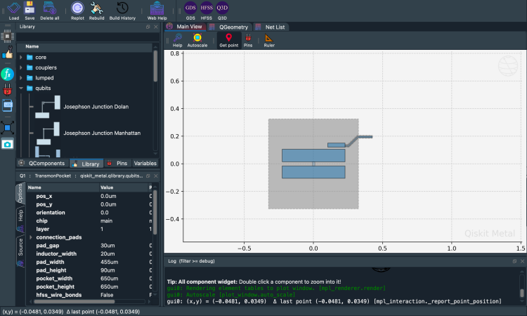
[9]:
# Select a QComponent to create (The QComponent is a python class named `TransmonPocket`)
from qiskit_metal.qlibrary.qubits.transmon_pocket import TransmonPocket


q1 = TransmonPocket(
    design, "Q1", options=dict(connection_pads=dict(a=dict()))
)  # Create a new Transmon Pocket object with name 'Q1'
gui.rebuild()  # rebuild the design and plot

gui.edit_component("Q1")  # set Q1 as the editable component
gui.autoscale()  # resize GUI to see QComponent
Finally, you can inspect the component object directly. This prints useful information — including component type, name, and the resolved parameters.
[10]:
q1 # print Q1 information
[10]:
name:    Q1
class:   TransmonPocket
options:
  'pos_x'             : '0.0um',
  'pos_y'             : '0.0um',
  'orientation'       : '0.0',
  'chip'              : 'main',
  'layer'             : '1',
  'connection_pads'   : {
       'a'                 : {
            'pad_gap'           : '15um',
            'pad_width'         : '125um',
            'pad_height'        : '30um',
            'pad_cpw_shift'     : '5um',
            'pad_cpw_extent'    : '25um',
            'cpw_width'         : 'cpw_width',
            'cpw_gap'           : 'cpw_gap',
            'cpw_extend'        : '100um',
            'pocket_extent'     : '5um',
            'pocket_rise'       : '65um',
            'loc_W'             : '+1',
            'loc_H'             : '+1',
                             },
                        },
  'pad_gap'           : '30um',
  'inductor_width'    : '20um',
  'pad_width'         : '455um',
  'pad_height'        : '90um',
  'pocket_width'      : '650um',
  'pocket_height'     : '650um',
  'hfss_wire_bonds'   : False,
  'q3d_wire_bonds'    : False,
  'aedt_q3d_wire_bonds': False,
  'aedt_hfss_wire_bonds': False,
  'hfss_inductance'   : '10nH',
  'hfss_capacitance'  : 0,
  'hfss_resistance'   : 0,
  'hfss_mesh_kw_jj'   : 7e-06,
  'q3d_inductance'    : '10nH',
  'q3d_capacitance'   : 0,
  'q3d_resistance'    : 0,
  'q3d_mesh_kw_jj'    : 7e-06,
  'gds_cell_name'     : 'my_other_junction',
  'aedt_q3d_inductance': 1e-08,
  'aedt_q3d_capacitance': 0,
  'aedt_hfss_inductance': 1e-08,
  'aedt_hfss_capacitance': 0,
module:  qiskit_metal.qlibrary.qubits.transmon_pocket
id:      1
[ ]:
gui.screenshot() # screenshot of the design in GUI
What are the default options?
The QComponent comes with some default options like the length of the pads for our transmon pocket.
Options are parsed internally by Qiskit Metal via the component’s
makefunction.You can change option parameters from the gui or the script api.
[11]:
%metal_print How do I edit options? API or GUI
Updating and Viewing Your Design in the GUI 👀
You can now use the Metal GUI to edit, plot, and modify quantum components. Equivalently, you can also do everything from the Jupyter Notebooks/Python scripts (which call the Python API directly). The GUI is just calling the Python API for you.
*You must use a string when setting options!
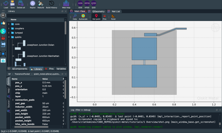
[12]:
# Change options
q1.options.pos_x = "0.5 mm"
q1.options.pos_y = "0.25 mm"
q1.options.pad_height = "225 um"
q1.options.pad_width = "250 um"
q1.options.pad_gap = "50 um"
Rebuild: This step re-generates all shapes for the components in the current design and syncs them with what you see in the Metal GUI window.
[13]:
gui.rebuild()  # Update the component geometry, since we changed the options

# Get a list of all the qcomponents in QDesign and then zoom on them.
all_component_names = design.components.keys()

gui.zoom_on_components(all_component_names)

# An alternate way to view within GUI. If want to try it, remove the "#" from the beginning of line.
# gui.autoscale() #resize GUI
[18]:
gui.screenshot() # screenshot of the design in GUI
Closing the Qiskit Metal GUI
[ ]:
# gui.main_window.close()
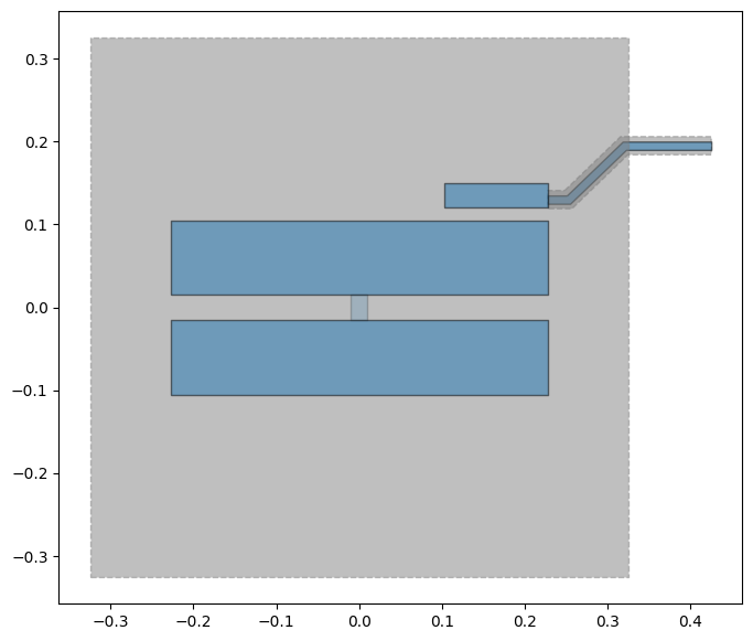
Following along without the Qt GUI
Everything we just did works without MetalGUI — the design, components, and analyses are all Qt-free. Use qm.view(design) to display the design inline in any matplotlib-aware environment (Jupyter, Colab, Binder, or a plain Python script).
Here’s the headless equivalent of the workflow above:
[15]:
%matplotlib inline
[16]:
import qiskit_metal as qm
from qiskit_metal import Dict, designs
from qiskit_metal.qlibrary.qubits.transmon_pocket import TransmonPocket

# Same design as above — no Qt needed
design = designs.DesignPlanar()
TransmonPocket(
    design,
    "Q1",
    options=Dict(connection_pads=Dict(a=Dict())),
)

fig = qm.view(design)
fig  # inline-display in Jupyter; fig.savefig("...") to write to file
[16]:

For a new kernel session if you want you can also try to run in interactive mode, instead of %matplotlib inline, `
[18]:
%matplotlib widget
[19]:
fig = qm.view(design)
fig  # inline-display in Jupyter; fig.savefig("...") to write to file
[19]:
For more information, review the Introduction to Quantum Computing and Quantum Hardware lectures below
|
Lecture Video | Lecture Notes | Lab |
|
Lecture Video | Lecture Notes | Lab |
|
Lecture Video | Lecture Notes | Lab |
|
Lecture Video | Lecture Notes | Lab |
|
Lecture Video | Lecture Notes | Lab |
|
Lecture Video | Lecture Notes | Lab |