Note
This page was generated from tut/3-Renderers/3.2-Export-your-design-to-GDS.ipynb.
3.2 Export your design to GDS
💡 Using this tutorial without the Qt GUI
This tutorial uses the desktop
MetalGUI. To follow along on Colab, Binder, JupyterHub, or any environment where Qt isn’t available, replace any ``gui.rebuild()`` / ``gui.screenshot()`` call with ``qm.view(design)`` — it renders the design to a matplotlibFigureyou can display inline or save withfig.savefig(...).See 1.1 Quick start for a complete runnable walkthrough and
`docs/headless-usage.rst<../../docs/headless-usage.rst>`__ for the full reference.
For convenience, let’s begin by enabling automatic reloading of modules when they change.
What does export_to_gds() put in my GDS file?
The cells below walk through the complete export pipeline:
Metal geometry (ground plane, qubit pockets, CPW traces) on the component’s
layernumberJunction cells imported from an external GDS file and placed at each junction slot
Cheesing geometry (hole grid and keepout regions) on configurable sub-layers
Positive or negative mask output, selectable per layer
By the end you will be able to: export a full or partial design, inspect the layer/datatype structure, configure cheesing and mask polarity, and use the fabricate flag to strip debug intermediates from the final file.
Import Qiskit Metal
[1]:
import qiskit_metal as metal
import qiskit_metal as qm
from qiskit_metal import designs, draw
from qiskit_metal import Dict, Headings
from qiskit_metal.qlibrary.qubits.transmon_pocket import TransmonPocket
from qiskit_metal.qlibrary.qubits.transmon_cross import TransmonCross
[2]:
design = designs.DesignPlanar()
gui = qm.gui(design)
qm.view(design); gui.rebuild(), gui.screenshot(), gui.edit_component(...) work as in the desktop GUI.For the full desktop experience (Qt window, dockable panels):
pip install 'quantum-metal[gui]' and re-import.[3]:
design.overwrite_enabled = True
design.delete_all_components()
gui.rebuild()  # refresh
[3]:
[4]:
Headings.h1("Populate QDesign to demonstrate exporting to GDS format.")
Populate QDesign to demonstrate exporting to GDS format.
[5]:
from qiskit_metal.qlibrary.qubits.transmon_pocket import TransmonPocket

# Allow running the same cell here multiple times to overwrite changes.
design.overwrite_enabled = True

## Custom options for all the transmons.
options = dict(
    # Some options we want to modify from the defaults.
    # (see below for defaults)
    pad_gap="80 um",
    pad_width="425 um",
    pocket_height="650um",
    # Adding 4 connectors (see below for defaults)
    connection_pads=dict(
        a=dict(loc_W=+1, loc_H=+1),
        b=dict(loc_W=-1, loc_H=+1, pad_height="30um"),
        c=dict(loc_W=+1, loc_H=-1, pad_width="200um"),
        d=dict(loc_W=-1, loc_H=-1, pad_height="50um"),
    ),
)
``gds_cell_name`` — each
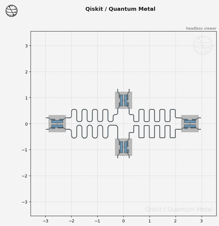
TransmonPocketcarries agds_cell_nameoption that tells the GDS renderer which cell to pull fromgds.options.path_filenameand place at the junction slot. Using different names here (FakeJunction_01, _02, my_other_junction) lets you see all three cells in one export and verify orientation.
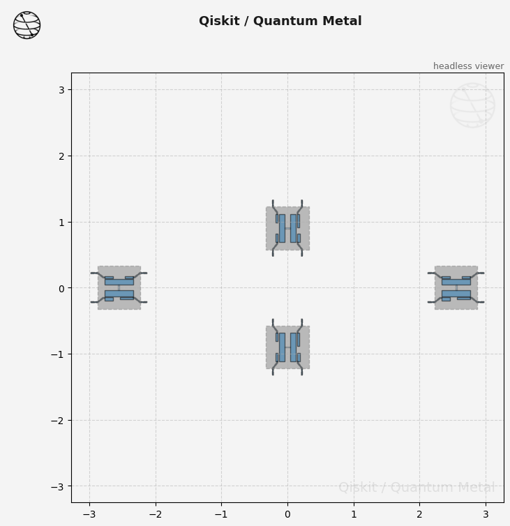
[6]:
## Create 4 TransmonPockets

# For variety and demonstartion, use different gds_cell_names.
q1 = TransmonPocket(
    design,
    "Q1",
    options=dict(
        pos_x="+2.55mm", pos_y="+0.0mm", gds_cell_name="FakeJunction_02", **options
    ),
)
q2 = TransmonPocket(
    design,
    "Q2",
    options=dict(
        pos_x="+0.0mm",
        pos_y="-0.9mm",
        orientation="90",
        gds_cell_name="FakeJunction_01",
        **options,
    ),
)
q3 = TransmonPocket(
    design,
    "Q3",
    options=dict(
        pos_x="-2.55mm", pos_y="+0.0mm", gds_cell_name="FakeJunction_01", **options
    ),
)
q4 = TransmonPocket(
    design,
    "Q4",
    options=dict(
        pos_x="+0.0mm",
        pos_y="+0.9mm",
        orientation="90",
        gds_cell_name="my_other_junction",
        **options,
    ),
)

## Rebuild the design
gui.rebuild()
gui.autoscale()
[6]:

[7]:
gui.screenshot()
# Headless alternative: qm.view(design)
Connecting QPins with coplanar waveguides (CPWs) as described in earlier notebooks.
[8]:
from qiskit_metal.qlibrary.tlines.meandered import RouteMeander

RouteMeander.get_template_options(design)

options = Dict(meander=Dict(lead_start="0.1mm", lead_end="0.1mm", asymmetry="0 um"))


def connect(
    component_name: str,
    component1: str,
    pin1: str,
    component2: str,
    pin2: str,
    length: str,
    asymmetry="0 um",
    flip=False,
    fillet="50um",
):
    """Connect two pins with a CPW."""
    myoptions = Dict(
        fillet=fillet,
        pin_inputs=Dict(
            start_pin=Dict(component=component1, pin=pin1),
            end_pin=Dict(component=component2, pin=pin2),
        ),
        lead=Dict(start_straight="0.13mm", end_straight="0.13mm"),
        total_length=length,
    )
    myoptions.update(options)
    myoptions.meander.asymmetry = asymmetry
    myoptions.meander.lead_direction_inverted = "true" if flip else "false"
    return RouteMeander(design, component_name, myoptions)


asym = 90

# For variety in output, use different fillet values.
cpw1 = connect("cpw1", "Q1", "d", "Q2", "c", "5.7 mm", f"+{asym}um", fillet="25um")
cpw2 = connect(
    "cpw2", "Q3", "c", "Q2", "a", "5.4 mm", f"-{asym}um", flip=True, fillet="100um"
)
cpw3 = connect("cpw3", "Q3", "a", "Q4", "b", "5.3 mm", f"+{asym}um", fillet="75um")
cpw4 = connect("cpw4", "Q1", "b", "Q4", "d", "5.5 mm", f"-{asym}um", flip=True)

gui.rebuild()
gui.autoscale()
[8]:
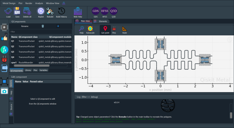
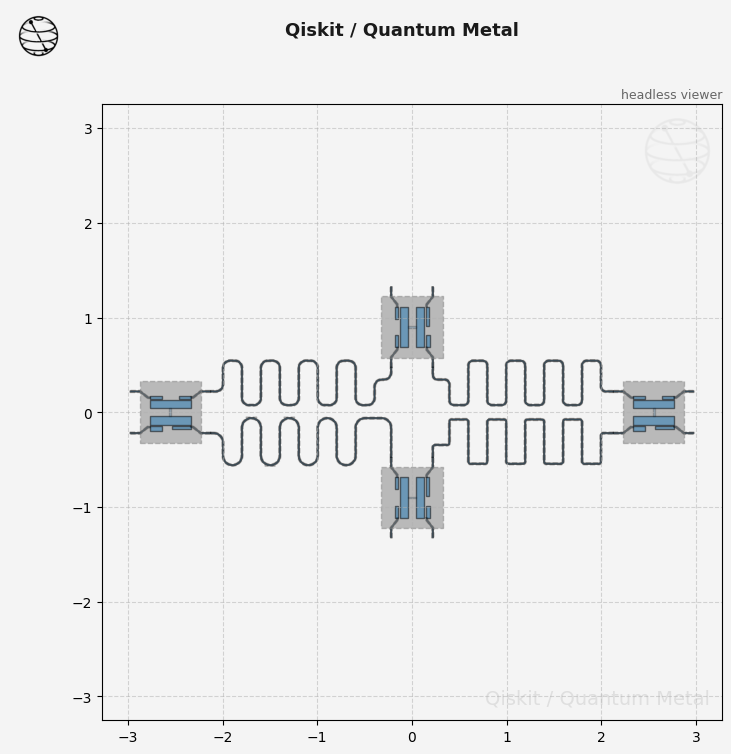
[9]:
gui.screenshot()
# Headless alternative: qm.view(design)
[10]:
Headings.h1("Exporting to a GDS file.")
Exporting to a GDS file.
[11]:
# QDesign registers GDS renderer during init of QDesign.
a_gds = design.renderers.gds
# An alternate way to invoke gds commands without using a_gds:
# design.renderers.gds.export_to_gds()

# Show the options for GDS
a_gds.options
[11]:
{'short_segments_to_not_fillet': 'True',
 'check_short_segments_by_scaling_fillet': '2.0',
 'gds_unit': 0.001,
 'ground_plane': 'True',
 'negative_mask': {'main': []},
 'fabricate': 'False',
 'corners': 'natural',
 'tolerance': '0.00001',
 'precision': '0.000000001',
 'width_LineString': '10um',
 'path_filename': '../resources/Fake_Junctions.GDS',
 'junction_pad_overlap': '5um',
 'max_points': '199',
 'cheese': {'datatype': '100',
  'shape': '0',
  'cheese_0_x': '25um',
  'cheese_0_y': '25um',
  'cheese_1_radius': '100um',
  'view_in_file': {'main': {1: True}},
  'delta_x': '100um',
  'delta_y': '100um',
  'edge_nocheese': '200um'},
 'no_cheese': {'datatype': '99',
  'buffer': '25um',
  'cap_style': '2',
  'join_style': '2',
  'view_in_file': {'main': {1: True}}},
 'bounding_box_scale_x': '1.2',
 'bounding_box_scale_y': '1.2'}
Will export_to_gds() add datatype for Polygon and Flexpath to my GDS file.
Yes. If you see a datatype being added to your positive mask, datatype=10 means a Polygon was added to the layer, datatype=11 means Flexpath was added to the layer. However, for each layer that has a negative mask, due to boolean subtract command done by export_to_gds, the 10 and 11 datatypes will not be in the gds file.
For positive mask, datatype=0 is for the ground plane.
To make junction table work correctly, GDS Renderer needs a correct path to a gds file, which has cells.
Each cell is a junction, to be placed, in a Transmon. A sample gds file is provided in directory qiskit_metal/tutorials/resources. There are three cells with names “Fake_Junction_01”, “Fake_Junction_01”, and “my_other_junction”. The default name used by GDS Render is “my_other_junction”. If you want to customize and select a junction, through the QComponent’s options, you can pass it when a qcomponent is being added to QDesign.
If your added junctions to a qcomponent.
The junctions are imported from file at gds.options.path_filename. The cell from path_filename which is denoted by TransmonPocket.options.gds_cell_name is imported and placed at location determined by the qcomponent developer. The method export_to_gds will place the imported cell at the same layers which are identified in the file at gds.options.path_filename.
[12]:
a_gds.options["path_filename"] = "../resources/Fake_Junctions.GDS"
Do you want GDS Renderer to fix any short-segments in your QDesign when using fillet?’
[13]:
# If you have a fillet_value and there are LineSegments that are shorter than 2*fillet_value,
# When true, the short segments will not be fillet'd.
a_gds.options["short_segments_to_not_fillet"] = "False"
[14]:
scale_fillet = 2.0
a_gds.options["check_short_segments_by_scaling_fillet"] = scale_fillet
What criteria will be used for identifying a short segment?
If a segment is smaller than (fillet length * scale_fillet)
What if a segment of LineString has few short segments?
If option ‘short_segments_to_not_fillet’ == ‘True’, QGDSRenderer will break the LineString into shorter Linestrings to make smaller LineStrings that will be either fillet’d or not, based on if the segment is short.
[15]:
# If you want to have the short segments not be fillet'd.
a_gds.options["short_segments_to_not_fillet"] = "True"
[16]:
# Export to a GDS formatted file for all components in design.
# def export_to_gds(self, file_name: str, highlight_qcomponents: list = []) -> int:

a_gds.export_to_gds("GDS QRenderer Notebook.gds")
# You can also specify a different path. Example:
#   a_gds.export_to_gds("../../../gds-files/GDS QRenderer Notebook.gds")
08:56PM 37s WARNING [import_junction_gds_file]: Not able to find file:"../resources/Fake_Junctions.GDS". Not used to replace junction. Checked directory:"/Users/zlatkominev/CODE_REPOS/quantum_hardware/qiskit-metal/docs/tut/resources".
[16]:
1
[17]:
# Export a GDS file which contains only few components.

# You will probably want to put the exported file in a specific directory.
# Please give the full path for output.
a_gds.export_to_gds(
    "four_qcomponents.gds", highlight_qcomponents=["cpw1", "cpw4", "Q1", "Q3"]
)
08:56PM 38s WARNING [import_junction_gds_file]: Not able to find file:"../resources/Fake_Junctions.GDS". Not used to replace junction. Checked directory:"/Users/zlatkominev/CODE_REPOS/quantum_hardware/qiskit-metal/docs/tut/resources".
[17]:
1
[18]:
# Export a GDS file using explicit path and cpw1.name vs typing string.
# You will probably want to put the exported file in a specific directory.
# Please give the full path for output.
a_gds.export_to_gds(
    "four_same_qcomponents.gds",
    highlight_qcomponents=[cpw1.name, "cpw4", q1.name, "Q3"],
)
08:56PM 38s WARNING [import_junction_gds_file]: Not able to find file:"../resources/Fake_Junctions.GDS". Not used to replace junction. Checked directory:"/Users/zlatkominev/CODE_REPOS/quantum_hardware/qiskit-metal/docs/tut/resources".
[18]:
1
[19]:
Headings.h1("QUESTION: Where is the geometry of a QComponent placed?")
QUESTION: Where is the geometry of a QComponent placed?
Answer: QGeometry tables!
QGeometry tables are covered in detail in 2.4 — QRenderer Introduction. The short answer: every polygon, path, and junction slot that a component creates lands in the poly, path, or junction table respectively, and all renderers read from those tables on export.
[20]:
Headings.h1('What does GDS do with "junction" table?')
What does GDS do with "junction" table?
The junction table is handled differently by each QRenderer.
GDS QRenderer gets a cell, with the name, equal to “gds_cell_name” and places the cell into the QDesign before exporting the entire QDesign to GDS. In file: a_gds.options['path_filename'] = '../resources/Fake_Junctions.GDS', the gds_cell_name is searched. The cell is placed into QDesign using LINESTRING and width information.
The cell within “path_filename”, should be “x-axis” aligned and then GDS rotates based on LineString. The LineString should be two vertexes and it denotes two things.
The midpoint of segment is the center of cell.
The angle made by (second tuple - fist tuple), for delta y/ delta x, is used to rotate the cell.
When the cell from default_options.path_filename does not fit the width of LineString,
QGDSRender will create two pads and add to cell, which is denoted in junction table, to fill the width of LineString. The length of the additional pads is the value of “width” from the junction table.
The option
a_gds.options["junction_pad_overlap"]='5um'is the amount the new pads will overlap the cell. The final width of the cell plus two pads is equal to the magnitude of LineString.
[21]:
# View every entry in junction table.
design.qgeometry.tables["junction"]
[21]:
| component | name | geometry | layer | subtract | helper | chip | width | hfss_inductance | hfss_capacitance | ... | hfss_mesh_kw_jj | q3d_inductance | q3d_capacitance | q3d_resistance | q3d_mesh_kw_jj | gds_cell_name | aedt_q3d_inductance | aedt_q3d_capacitance | aedt_hfss_inductance | aedt_hfss_capacitance | |
|---|---|---|---|---|---|---|---|---|---|---|---|---|---|---|---|---|---|---|---|---|---|
| 0 | 1 | rect_jj | LINESTRING (2.55 -0.04, 2.55 0.04) | 1 | False | False | main | 0.02 | 10nH | 0 | ... | 0.000007 | 10nH | 0 | 0 | 0.000007 | FakeJunction_02 | 1.000000e-08 | 0 | 1.000000e-08 | 0 |
| 1 | 2 | rect_jj | LINESTRING (0.04 -0.9, -0.04 -0.9) | 1 | False | False | main | 0.02 | 10nH | 0 | ... | 0.000007 | 10nH | 0 | 0 | 0.000007 | FakeJunction_01 | 1.000000e-08 | 0 | 1.000000e-08 | 0 |
| 2 | 3 | rect_jj | LINESTRING (-2.55 -0.04, -2.55 0.04) | 1 | False | False | main | 0.02 | 10nH | 0 | ... | 0.000007 | 10nH | 0 | 0 | 0.000007 | FakeJunction_01 | 1.000000e-08 | 0 | 1.000000e-08 | 0 |
| 3 | 4 | rect_jj | LINESTRING (0.04 0.9, -0.04 0.9) | 1 | False | False | main | 0.02 | 10nH | 0 | ... | 0.000007 | 10nH | 0 | 0 | 0.000007 | my_other_junction | 1.000000e-08 | 0 | 1.000000e-08 | 0 |
4 rows × 21 columns
[22]:
# View the juction table for component "q1".

q1.qgeometry_table("junction")
[22]:
| component | name | geometry | layer | subtract | helper | chip | width | hfss_inductance | hfss_capacitance | ... | hfss_mesh_kw_jj | q3d_inductance | q3d_capacitance | q3d_resistance | q3d_mesh_kw_jj | gds_cell_name | aedt_q3d_inductance | aedt_q3d_capacitance | aedt_hfss_inductance | aedt_hfss_capacitance | |
|---|---|---|---|---|---|---|---|---|---|---|---|---|---|---|---|---|---|---|---|---|---|
| 0 | 1 | rect_jj | LINESTRING (2.55 -0.04, 2.55 0.04) | 1 | False | False | main | 0.02 | 10nH | 0 | ... | 0.000007 | 10nH | 0 | 0 | 0.000007 | FakeJunction_02 | 1.000000e-08 | 0 | 1.000000e-08 | 0 |
1 rows × 21 columns
Geometric boundary of a QComponent
q1.qgeometry_bounds() returns (minx, miny, maxx, maxy) for all geometry belonging to that component. Covered in full in 2.4 — QRenderer Introduction.
[23]:
# The current value of all the options for GDS QRenderer.
a_gds.options
[23]:
{'short_segments_to_not_fillet': 'True',
 'check_short_segments_by_scaling_fillet': 2.0,
 'gds_unit': 0.001,
 'ground_plane': 'True',
 'negative_mask': {'main': []},
 'fabricate': 'False',
 'corners': 'natural',
 'tolerance': '0.00001',
 'precision': '0.000000001',
 'width_LineString': '10um',
 'path_filename': '../resources/Fake_Junctions.GDS',
 'junction_pad_overlap': '5um',
 'max_points': '199',
 'cheese': {'datatype': '100',
  'shape': '0',
  'cheese_0_x': '25um',
  'cheese_0_y': '25um',
  'cheese_1_radius': '100um',
  'view_in_file': {'main': {1: True}},
  'delta_x': '100um',
  'delta_y': '100um',
  'edge_nocheese': '200um'},
 'no_cheese': {'datatype': '99',
  'buffer': '25um',
  'cap_style': '2',
  'join_style': '2',
  'view_in_file': {'main': {1: True}}},
 'bounding_box_scale_x': '1.2',
 'bounding_box_scale_y': '1.2'}
Number of vertices for linestrings.
The option max_points has default of 199. You can set it to a number no higher than 8191.
[24]:
### For demo, set max_points to 8191 and look at the GDS output.
a_gds.options["max_points"] = "8191"
a_gds.export_to_gds("GDS QRenderer Notebook maxpoints8191.gds")
08:56PM 38s WARNING [import_junction_gds_file]: Not able to find file:"../resources/Fake_Junctions.GDS". Not used to replace junction. Checked directory:"/Users/zlatkominev/CODE_REPOS/quantum_hardware/qiskit-metal/docs/tut/resources".
[24]:
1
Changing options ‘precision’ vs ‘tolerance’ ratio can impact how fillet will look.
The below numbers are used to create a gdstk.FlexPath when there is a fillet value in QGeometry table.
bend_radius – Bend radii for each path when corners is ‘circular bend’. It has no effect for other corner types. QGDSRender uses ‘circular bend’ as a default for corners. The fillet value used here.
Ensure that tolerance > precision.
tolerance (number) – Tolerance used to draw the paths and calculate joins.
precision (number) – Precision for rounding the coordinates of vertices when fracturing the final polygonal boundary.
[25]:
# Restore previous example.
a_gds.options["max_points"] = "199"

# For Demo, change tolerance value.
a_gds.options["tolerance"] = "0.01"
# This exported file will not look as desired.
a_gds.export_to_gds("GDS QRenderer Notebook change tolerance.gds")
08:56PM 38s WARNING [import_junction_gds_file]: Not able to find file:"../resources/Fake_Junctions.GDS". Not used to replace junction. Checked directory:"/Users/zlatkominev/CODE_REPOS/quantum_hardware/qiskit-metal/docs/tut/resources".
[25]:
1
[26]:
# change it back to was it was.
a_gds.options["tolerance"] = "0.00001"
[27]:
Headings.h1("Layer numbers: cheese and mask")
Layer numbers: cheese and mask
What can I control by layer number?
positive mask
negative mask
cheese
no_cheese
If you wanted cheese or no_cheese in the GDS file.
The reason you choose to use cheesing is up to the developer. There are considerations for both manufacturing and EM design. This refers to the holes in the output GDS ground plane (cheese = holes). From an EM stand-point https://www.degruyter.com/document/doi/10.1515/psr-2017-8000/html.
Cheesing refers to the holes added to the chip. The “cheese” output will correspond to the mask (positive or negative) selected. Both cheese and no_cheese output can be generated for any layer. You can choose to add the no_cheese to the exported GDS file; adding no_cheese information in GDS file, is just to show the intermediate step.
In the cheese dict, edge_nocheese option denotes a buffer around the perimeter of the chip. You can identify which layer has the cheesing by using the key view_in_file. To identify a datatype to store the geometry for cheesing, edit the key named datatype.
The option no_cheese can be thought of as a “keep-out” region for cheesing. Based on the components on the chip, a no-cheese region is determined. The no_cheese region is created by adding a buffer around all the components. In no_cheese dict, there is a key called buffer, that denotes the size around all the components for no_cheese. Even if view_in_file may be True for cheese dict, user can make it false for no_cheese dict. If the user wants to view the no_cheese region in the GDS output, keep it as True for each layer you are interested it.
The location of cheesing is determined by
generating a grid of holes for the size of chip
subtract the no_cheese region
subtract the edge_nocheese region
The method export_to_gds, uses the datatype in cheese dict, default is 100, and no_cheese dict, default is 99; then uses few extra datatypes by adding one or two. The extra datatypes are to show some intermediate steps. If you choose to view_in_file, then you will see cheese or no-cheese in the gds file.
TOP_chipname_layernumber_one_hole is a cell with just one hole. The rest of the holes are made as a reference from the one hole. The hole is placed with datatype_cheese+2. This is expected to change when we agree to some convention.
TOP_chipname_layernumber_NoCheese_datatype is a cell that holds the “keep-out” region for cheesing.
TOP_chipname_layernumber_Cheese_datatype is a cell that holds the cheesing region.
TOP_chipname_layernumber holds the geometry taken from Metal GUI.
TOP_chipname_layernumber_Cheese_diff is a cell that holds the difference between grid of holes on chip, minus the no_cheese region. It is placed in datatype_cheese+1. This is expected to change when we agree to some convention.
For negative mask: TOP_chipname_layernumber_Cheese_diff is placed under TOP_chipname_layernumber.
For positive mask: TOP_chipname_layernumber_Cheese_diff is subtracted from ground and placed under TOP_chipname_layernumber.
Changing Cheesing options
There are two dicts in default_options for cheesing. One for selecting the no_cheese (keep-out region) for cheesing, the other for cheesing. Use them to determine if you would like the cheesing cell and the no_cheese cell to be added to the GDS file.
To create the no-cheese region, we take the existing components and add a buffer around the perimeter. The size of the buffer is an option.
The output of the cells can be placed with a data type. The user can select a different data type for both the no-cheese region and the cheese region.
Regarding the cheese option, there is room for expansion, presently, the shape that available for a hole is a shape=0, which is a square.
The present placement of holes allows the user to apply edge_nocheese to the perimeter of the chip. This allows the user to place holes at a perimeter smaller than the chip size. Then a grid of holes is made using delta_x and delta_y.
[28]:
a_gds.options.no_cheese
[28]:
{'datatype': '99',
 'buffer': '25um',
 'cap_style': '2',
 'join_style': '2',
 'view_in_file': {'main': {1: True}}}
[29]:
a_gds.options.cheese
[29]:
{'datatype': '100',
 'shape': '0',
 'cheese_0_x': '25um',
 'cheese_0_y': '25um',
 'cheese_1_radius': '100um',
 'view_in_file': {'main': {1: True}},
 'delta_x': '100um',
 'delta_y': '100um',
 'edge_nocheese': '200um'}
There is a dict option called view_in_file that denotes if the cells are added to GDS file. The first sub-option is the chip name, the second sub-option is layer number, the third sub-option is bool True/False.
In our example, the chip is ‘main’ and the layer is 1. We allow for expansion for multiple chips, and multiple ground layers.
[30]:
a_gds.options["cheese"]["view_in_file"]["main"][1] = True
a_gds.options["no_cheese"]["view_in_file"]["main"][1] = True
a_gds.export_to_gds("GDS QRender_cheese_keepout.gds")
08:56PM 39s WARNING [import_junction_gds_file]: Not able to find file:"../resources/Fake_Junctions.GDS". Not used to replace junction. Checked directory:"/Users/zlatkominev/CODE_REPOS/quantum_hardware/qiskit-metal/docs/tut/resources".
[30]:
1
[31]:
a_gds.options["cheese"]["view_in_file"]["main"][1] = True
a_gds.options["no_cheese"]["view_in_file"]["main"][1] = False
a_gds.export_to_gds("GDS QRender_cheese_only.gds")
08:56PM 39s WARNING [import_junction_gds_file]: Not able to find file:"../resources/Fake_Junctions.GDS". Not used to replace junction. Checked directory:"/Users/zlatkominev/CODE_REPOS/quantum_hardware/qiskit-metal/docs/tut/resources".
[31]:
1
[32]:
# For example, just move the cpws to layer=14.
cpw1.options.layer = 14
cpw2.options.layer = 14
cpw3.options.layer = 14
cpw4.options.layer = 14
[33]:
gui.rebuild()

# Get a list of all the qcomponents in QDesign and then zoom on them.
all_component_names = design.components.keys()
gui.zoom_on_components(all_component_names)
# Headless alternative: qm.view(design, components=list(all_component_names))
Ignoring fixed y limits to fulfill fixed data aspect with adjustable data limits.
[33]:
[34]:
gui.screenshot()
Ignoring fixed y limits to fulfill fixed data aspect with adjustable data limits.

[35]:
# Turn on/off keep-out and cheesing.
a_gds.options["cheese"]["view_in_file"]["main"][1] = True
a_gds.options["no_cheese"]["view_in_file"]["main"][1] = True
a_gds.options["cheese"]["view_in_file"]["main"][14] = True
a_gds.options["no_cheese"]["view_in_file"]["main"][14] = True
If you want a positive and/or negative masks.
User can request a positive or negative mask by chip-name and layer-number. The default is to use a positive mask. If user wants to use a negative mask, then just identify the layers that should be a negative mask. The user is allowed to mix the output per chip, per layer. Particularly, a chip can have both positive and negative masks; the granularity is by layer. This is exemplified in this notebook by editing option “negative_mask”. This feature was implemented for, potential use, for “flip-chip”.
[36]:
# Export GDS file with negative masks for layers 1 and 14.
a_gds.options["negative_mask"] = Dict(main=[1, 14])
a_gds.export_to_gds("GDS QRenderer Notebook_neg_mask_for_layer_1_14.gds")
08:56PM 40s WARNING [import_junction_gds_file]: Not able to find file:"../resources/Fake_Junctions.GDS". Not used to replace junction. Checked directory:"/Users/zlatkominev/CODE_REPOS/quantum_hardware/qiskit-metal/docs/tut/resources".
[36]:
1
[37]:
# Export GDS files with positive mask for layer 1 and negative mask for layer 14.
a_gds.options["negative_mask"] = Dict(main=[14])
a_gds.export_to_gds("GDS QRenderer Notebook_neg_mask_for_layer_14.gds")
08:56PM 40s WARNING [import_junction_gds_file]: Not able to find file:"../resources/Fake_Junctions.GDS". Not used to replace junction. Checked directory:"/Users/zlatkominev/CODE_REPOS/quantum_hardware/qiskit-metal/docs/tut/resources".
[37]:
1
[38]:
# Load and inspect the exported GDS.
# show=True renders the design as an embedded SVG in this cell output
# (the image saves with the notebook — no external file needed).
# scale: increase for larger chips or more detail (default 100)
# width: display width in pixels (default 800)

import gdstk

lib = gdstk.read_gds("GDS QRenderer Notebook_neg_mask_for_layer_1_14.gds")
a_gds.debug_summarize_gds_library(lib, show=True, scale=100, width=900)

# lib = gdstk.read_gds("GDS QRenderer Notebook_neg_mask_for_layer_14.gds")
# a_gds.debug_summarize_gds_library(lib, show=True, scale=100, width=900)
| Layer | DType | Description | Polygons | Paths | |
|---|---|---|---|---|---|
| 1 | 0 | metal (boolean result) | 4 poly | 0 paths | |
| 1 | 99 | 4 poly | 0 paths | ||
| 1 | 101 | 4618 poly | 0 paths | ||
| 1 | 102 | 1 poly | 0 paths | ||
| 14 | 0 | metal (boolean result) | 64 poly | 0 paths | |
| 14 | 99 | 4 poly | 0 paths | ||
| 14 | 101 | 4640 poly | 0 paths | ||
| 14 | 102 | 1 poly | 0 paths |
=== GDS LIBRARY SUMMARY ===
name:      library
unit:      0.001
precision: 1e-09
cells:     10

CELLS:
  - TOP                            geom=True bbox=((-4.3125, -2.8125), (4.2124999999999995, 2.7125))
  - TOP_main                       geom=True bbox=((-4.3125, -2.8125), (4.2124999999999995, 2.7125))
  - TOP_main_1                     geom=True bbox=((-4.3125, -2.8125), (4.2124999999999995, 2.7125))
  - TOP_main_14                    geom=True bbox=((-4.3125, -2.8125), (4.2124999999999995, 2.7125))
  - TOP_main_1_NoCheese_99         geom=True bbox=((-3.0, -1.3499999999999999), (3.0, 1.3499999999999999))
  - TOP_main_14_NoCheese_99        geom=True bbox=((-2.15, -0.5941029999999999), (2.15, 0.580476))
  - TOP_main_1_one_hole            geom=True bbox=((-0.012499999999999999, -0.012499999999999999), (0.012499999999999999, 0.012499999999999999))
  - TOP_main_1_Cheese_diff         geom=True bbox=((-4.3125, -2.8125), (4.2124999999999995, 2.7125))
  - TOP_main_14_one_hole           geom=True bbox=((-0.012499999999999999, -0.012499999999999999), (0.012499999999999999, 0.012499999999999999))
  - TOP_main_14_Cheese_diff        geom=True bbox=((-4.3125, -2.8125), (4.2124999999999995, 2.7125))

LAYER / DATATYPE USAGE:
  layer  dtype   polys   paths
  -----  -----   -----   -----
      1      0       4       0
      1     99       4       0
      1    101    4618       0
      1    102       1       0
     14      0      64       0
     14     99       4       0
     14    101    4640       0
     14    102       1       0

=== END SUMMARY ===
[39]:
Headings.h1("Fabrication")
Fabrication
There is no universally accepted method to prepare for fabrication of a chip. If this flag is True, cells created as part of intermittent steps would not be in the gds file. For example cells with names similar to “TOP_main_1_NoCheese_99” , “TOP_main_1_one_hole” and “ground_main_1”.
[40]:
# By default, the fabrication flag is False.
a_gds.options["fabricate"] = "True"
[41]:
# Export GDS files with positive mask for layer 1 and negative mask for layer 14 with fabricate flag as True.
a_gds.options["negative_mask"] = Dict(main=[14])
a_gds.export_to_gds("GDS QRenderer Notebook_neg_mask_for_layer_14_fabricate.gds")
08:56PM 41s WARNING [import_junction_gds_file]: Not able to find file:"../resources/Fake_Junctions.GDS". Not used to replace junction. Checked directory:"/Users/zlatkominev/CODE_REPOS/quantum_hardware/qiskit-metal/docs/tut/resources".
[41]:
1
[42]:
# Load and inspect the exported GDS.
# Re-run the export cell above first if awesome_design.gds looks like an older design.
import gdstk

lib = gdstk.read_gds("GDS QRenderer Notebook_neg_mask_for_layer_14_fabricate.gds")

# show=True renders the design as an embedded SVG in this cell output
# (the image saves with the notebook — no external file needed).
# scale: increase for larger chips or more detail (default 100)
# width: display width in pixels (default 800)
a_gds.debug_summarize_gds_library(lib, show=True, scale=100, width=900)
[GDSTK] Missing referenced cell ground_main_1
[GDSTK] Missing referenced cell TOP_main_1_one_hole
[GDSTK] Missing referenced cell TOP_main_1_Cheese_diff
[GDSTK] Missing referenced cell TOP_main_14_one_hole
| Layer | DType | Description | Polygons | Paths | |
|---|---|---|---|---|---|
| 1 | 10 | component polygon input | 24 poly | 0 paths | |
| 1 | 11 | CPW FlexPath trace | 16 poly | 0 paths | |
| 1 | 100 | 3293 poly | 0 paths | ||
| 14 | 0 | metal (boolean result) | 64 poly | 0 paths | |
| 14 | 101 | 4640 poly | 0 paths |
=== GDS LIBRARY SUMMARY ===
name:      library
unit:      0.001
precision: 1e-09
cells:     6

CELLS:
  - TOP                            geom=True bbox=((-4.5, -3.0), (4.5, 3.0))
  - TOP_main                       geom=True bbox=((-4.5, -3.0), (4.5, 3.0))
  - TOP_main_1                     geom=True bbox=((-4.5, -3.0), (4.5, 3.0))
  - TOP_main_14                    geom=True bbox=((-4.3125, -2.8125), (4.2124999999999995, 2.7125))
  - TOP_main_1_Cheese_100          geom=True bbox=((-4.5, -3.0), (4.5, 3.0))
  - TOP_main_14_Cheese_diff        geom=True bbox=((-4.3125, -2.8125), (4.2124999999999995, 2.7125))

LAYER / DATATYPE USAGE:
  layer  dtype   polys   paths
  -----  -----   -----   -----
      1     10      24       0
      1     11      16       0
      1    100    3293       0
     14      0      64       0
     14    101    4640       0

=== END SUMMARY ===
Qiskit Metal Version
[43]:
metal.about();
Qiskit Metal        0.7.3

Basic
____________________________________
 Python              3.11.14 (main, Dec  5 2025, 21:28:33) [Clang 21.1.4 ]
 Platform            Darwin arm64
 Installation path   /Users/zlatkominev/CODE_REPOS/quantum_hardware/qiskit-metal/src/qiskit_metal

Packages
____________________________________
 Numpy               1.26.4
 Qutip               5.2.2

Rendering
____________________________________
 Matplotlib          3.10.8

GUI
____________________________________
 PySide6 version     6.10.1
 Qt version          6.10.1
 SIP version         Not installed

IBM Quantum Team
[44]:
# Uncomment to close the GUI window when done.
# The next section (junction import details) re-uses the same design
# and renderer — leave the GUI open if you want to keep inspecting the design.
# gui.main_window.close()
Deep dive: junction import and cheesing
The sections above covered the end-to-end export flow. The rest of this notebook goes deeper on two topics that often need tuning before tapeout:
Junction GDS files — how cells are imported, unit-rescaled, and placed
Cheesing geometry — what the algorithm produces and how to read the output layers
[45]:
gds = design.renderers.gds
gds.options.path_filename
[45]:
'../resources/Fake_Junctions.GDS'
[46]:
gds.options.path_filename = "../resources/Fake_Junctions.GDS"
[47]:
q1.options
[47]:
{'pos_x': '+2.55mm',
 'pos_y': '+0.0mm',
 'orientation': '0.0',
 'chip': 'main',
 'layer': '1',
 'connection_pads': {'a': {'pad_gap': '15um',
   'pad_width': '125um',
   'pad_height': '30um',
   'pad_cpw_shift': '5um',
   'pad_cpw_extent': '25um',
   'cpw_width': 'cpw_width',
   'cpw_gap': 'cpw_gap',
   'cpw_extend': '100um',
   'pocket_extent': '5um',
   'pocket_rise': '65um',
   'loc_W': 1,
   'loc_H': 1},
  'b': {'pad_gap': '15um',
   'pad_width': '125um',
   'pad_height': '30um',
   'pad_cpw_shift': '5um',
   'pad_cpw_extent': '25um',
   'cpw_width': 'cpw_width',
   'cpw_gap': 'cpw_gap',
   'cpw_extend': '100um',
   'pocket_extent': '5um',
   'pocket_rise': '65um',
   'loc_W': -1,
   'loc_H': 1},
  'c': {'pad_gap': '15um',
   'pad_width': '200um',
   'pad_height': '30um',
   'pad_cpw_shift': '5um',
   'pad_cpw_extent': '25um',
   'cpw_width': 'cpw_width',
   'cpw_gap': 'cpw_gap',
   'cpw_extend': '100um',
   'pocket_extent': '5um',
   'pocket_rise': '65um',
   'loc_W': 1,
   'loc_H': -1},
  'd': {'pad_gap': '15um',
   'pad_width': '125um',
   'pad_height': '50um',
   'pad_cpw_shift': '5um',
   'pad_cpw_extent': '25um',
   'cpw_width': 'cpw_width',
   'cpw_gap': 'cpw_gap',
   'cpw_extend': '100um',
   'pocket_extent': '5um',
   'pocket_rise': '65um',
   'loc_W': -1,
   'loc_H': -1}},
 'pad_gap': '80 um',
 'inductor_width': '20um',
 'pad_width': '425 um',
 'pad_height': '90um',
 'pocket_width': '650um',
 'pocket_height': '650um',
 'hfss_wire_bonds': False,
 'q3d_wire_bonds': False,
 'aedt_q3d_wire_bonds': False,
 'aedt_hfss_wire_bonds': False,
 'hfss_inductance': '10nH',
 'hfss_capacitance': 0,
 'hfss_resistance': 0,
 'hfss_mesh_kw_jj': 7e-06,
 'q3d_inductance': '10nH',
 'q3d_capacitance': 0,
 'q3d_resistance': 0,
 'q3d_mesh_kw_jj': 7e-06,
 'gds_cell_name': 'FakeJunction_02',
 'aedt_q3d_inductance': 1e-08,
 'aedt_q3d_capacitance': 0,
 'aedt_hfss_inductance': 1e-08,
 'aedt_hfss_capacitance': 0}
Note the GDS entry for the JJ cell name from a GDS external file
'gds_cell_name': 'FakeJunction_01'
This cell name is pulled from the file set in gds.options.path_filename and placed inside the qubit pocket on export.
Junction GDS unit convention Your junction GDS file can use any unit (
1e-6for µm,1e-9for nm, etc.). > The renderer reads the file’s ownunitfield and automatically rescales all > junction geometry so it lands at the correct physical size in the exported design. > You do not need to pre-convert your junction file to match the design’s unit (mm). > The only requirement is that coordinates inside the GDS file are consistent with > its declaredunit.
Josephon Junction GDS file path: gds.options.path_filename
Using your own junction GDS file
Set gds.options.path_filename to any GDS file that contains your junction cells. The renderer will:
Read the file and detect its unit (e.g.
1e-6for µm,1e-9for nm).Compute a scale factor
= junction_file_unit / design_unitand rescale all junction geometry so physical dimensions are preserved.Merge the scaled cells into the exported GDS — no manual unit conversion needed.
The example file resources/Fake_Junctions.GDS ships with the repo and contains three placeholder cells (in µm coordinates): FakeJunction_01, FakeJunction_02, and my_other_junction. Real fab junction files work exactly the same way as long as their GDS unit field matches the coordinate values inside them.
Common pitfall: if you author a junction GDS in a tool that writes coordinates > in nm but sets
unit=1e-6(µm), the cell will import at 1000× the intended size. > Always verify withgds.debug_summarize_gds_library()that junction cell bounding > boxes match expected physical dimensions after export.
[48]:
gds.lib
[48]:
<gdstk.Library at 0x30415e310>
[49]:
gds.options.path_filename = "../resources/Fake_Junctions.GDS"
gds.import_junction_gds_file(gds.lib)  # load into pour library
08:56PM 41s WARNING [import_junction_gds_file]: Not able to find file:"../resources/Fake_Junctions.GDS". Not used to replace junction. Checked directory:"/Users/zlatkominev/CODE_REPOS/quantum_hardware/qiskit-metal/docs/tut/resources".
[49]:
False
This function will read the file again, and print out the cells in it. It will also render the cells as an SVG inline if run in a Jupyter notebook.
[50]:
gds.show_imported_junction_gds() # Shows gds.imported_junction_gds
08:56PM 41s INFO [show_imported_junction_gds]: No junction gds file has been imported.
You can set it with `gds.options.path_filename = ...`
[51]:
# Disable cheesing output for this export.
# view_in_file controls whether cheese/no-cheese geometry appears in the GDS file.
# {1: False} = layer 1 present but suppress cheese holes from the output.
# Using Dict(main={}) triggers a warning — always specify layers explicitly.
gds.options.cheese.view_in_file = Dict(main={1: False})
gds.options.no_cheese.view_in_file = Dict(main={1: False})
[52]:
design.renderers.gds.export_to_gds("awesome_design.gds")
08:56PM 41s WARNING [import_junction_gds_file]: Not able to find file:"../resources/Fake_Junctions.GDS".  Not used to replace junction. Checked directory:"/Users/zlatkominev/CODE_REPOS/quantum_hardware/qiskit-metal/docs/tut/resources".
08:56PM 41s WARNING [_check_either_cheese]: layer=14 is not in chip=main either in no_cheese_view_in_file or cheese_view_in_file from self.options.
[52]:
1
[53]:
# Load and inspect the exported GDS.
# Re-run the export cell above first if awesome_design.gds looks like an older design.
import gdstk

lib = gdstk.read_gds("awesome_design.gds")

# show=True renders the design as an embedded SVG in this cell output
# (the image saves with the notebook — no external file needed).
# scale: increase for larger chips or more detail (default 100)
# width: display width in pixels (default 800)
a_gds.debug_summarize_gds_library(lib, show=True, scale=100, width=900)
| Layer | DType | Description | Polygons | Paths | |
|---|---|---|---|---|---|
| 1 | 0 | metal (boolean result) | 1 poly | 0 paths | |
| 1 | 10 | component polygon input | 24 poly | 0 paths | |
| 1 | 11 | CPW FlexPath trace | 16 poly | 0 paths | |
| 14 | 0 | metal (boolean result) | 64 poly | 0 paths |
=== GDS LIBRARY SUMMARY ===
name:      library
unit:      0.001
precision: 1e-09
cells:     5

CELLS:
  - TOP                            geom=True bbox=((-4.5, -3.0), (4.5, 3.0))
  - TOP_main                       geom=True bbox=((-4.5, -3.0), (4.5, 3.0))
  - TOP_main_1                     geom=True bbox=((-4.5, -3.0), (4.5, 3.0))
  - ground_main_1                  geom=True bbox=((-4.5, -3.0), (4.5, 3.0))
  - TOP_main_14                    geom=True bbox=((-2.125, -0.569103), (2.125, 0.555476))

LAYER / DATATYPE USAGE:
  layer  dtype   polys   paths
  -----  -----   -----   -----
      1      0       1       0
      1     10      24       0
      1     11      16       0
     14      0      64       0

=== END SUMMARY ===
[54]:
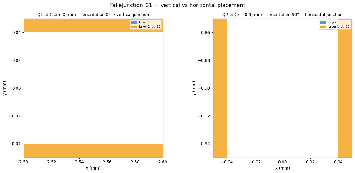
%matplotlib inline
[55]:
import matplotlib.pyplot as plt

# Q1 (orientation=0°)  → junction slot is vertical
# Q2 (orientation=90°) → junction slot is horizontal
# Both use FakeJunction_01 placed in the pocket centre.
fig, axes = plt.subplots(1, 2, figsize=(13, 6))
fig.suptitle("FakeJunction_01 — vertical vs horizontal placement", fontsize=13)

gds.plot_gds_zoom(
    lib,
    center_mm=(2.55, 0.0),
    span_mm=0.05,
    title="Q1 at (2.55, 0) mm — orientation 0° → vertical junction",
    ax=axes[0],
)
gds.plot_gds_zoom(
    lib,
    center_mm=(0.0, -0.9),
    span_mm=0.05,
    title="Q2 at (0, −0.9) mm — orientation 90° → horizontal junction",
    ax=axes[1],
)
plt.tight_layout()
# plt.close(fig)
# display(fig)
Status (v0.6.x+): The gdspy → gdstk migration is complete and validated. > Junction unit rescaling is applied automatically on import — junction cells from > any-unit GDS files (µm, nm, etc.) are scaled to the correct physical size in the > exported design. If you see junction geometry that looks too large or too small, > check that your junction GDS file’s
unitfield matches its internal coordinates > (see the note above), then re-export.
Appendix - GDS Cheesing: What It Is and How the Renderer Implements It
what “cheesing” means in mask design

Cheesing is the practice of punching a regular pattern of small holes into large metal areas (typically the ground plane). the holes make the metal look like swiss cheese, hence the name.
cheesing reduces fabrication issues such as:
film stress and cracking,
charging during lithography,
non-uniform etching,
rule violations caused by large continuous metal regions.
small holes mitigate these problems while leaving microwave behavior essentially unchanged.
the two components: cheese and no_cheese
cheesing relies on two option blocks in the renderer:
``cheese``: defines where holes should be created.
``no_cheese``: defines regions where holes are not allowed.
both have their own datatypes, sizes, spacing, and visibility settings:
gds.options.cheese
gds.options.no_cheese
how the renderer decides whether to cheese a layer
cheesing is activated only if the layer is marked in:
gds.options.cheese.view_in_file[chip][layer]
gds.options.no_cheese.view_in_file[chip][layer]
if neither entry exists for a given layer, cheesing is skipped.
step 1: determine ground-plane regions
before cheesing starts, the renderer constructs the metal ground plane geometry for each chip and layer:
shapes with
subtract=Truecut holes in the ground plane,shapes with
subtract=Falsesit on top of it.
this yields a unified understanding of the metal layout for the layer.
step 2: generate the “no-cheese” halo
this step computes regions where holes must not be placed.
it works by:
collecting all shapes that cut into the ground plane,
converting polylines into buffered polygons when needed,
unifying them into a single shape,
expanding them outward using
no_cheese.bufferto create a halo,clipping this halo to the chip boundary.
the resulting multipolygon forms a keep-out mask for cheesing.
step 3: tile the chip with holes
if cheesing is enabled, the renderer lays out a hole grid across the chip:
grid spacing is defined by
delta_xanddelta_y,hole size comes from
cheese_0_x,cheese_0_yorcheese_1_radius,hole shape is rectangular or circular based on
shape,holes near the chip edges (
edge_nocheese) are removed,holes that fall inside “no-cheese” regions are removed.
the resulting holes are added to gds on the appropriate datatype.
step 4: integrate holes into the final mask
cheese holes are merged differently depending on mask type:
positive mask: ground plane minus holes,
negative mask: inverse metal + hole logic.
this is done at the cell level so each chip_layer cell gets the correct geometry.
how to disable cheesing entirely
no renderer code needs modification. simply clear the visibility settings:
gds.options.cheese.view_in_file = Dict(main={})
gds.options.no_cheese.view_in_file = Dict(main={})
with no layers listed, cheesing logic never runs.
summary
the renderer’s cheesing pipeline is:
compute the ground plane,
compute no-cheese keep-out zones,
generate holes and filter them,
merge into positive or negative mask.
cheesing improves manufacturability while keeping electrical performance intact, and can be turned on/off per chip and per layer via simple configuration options.

[ ]:
For more information, review the Introduction to Quantum Computing and Quantum Hardware lectures below
|
Lecture Video | Lecture Notes | Lab |
|
Lecture Video | Lecture Notes | Lab |
|
Lecture Video | Lecture Notes | Lab |
|
Lecture Video | Lecture Notes | Lab |
|
Lecture Video | Lecture Notes | Lab |
|
Lecture Video | Lecture Notes | Lab |