Roadmap

Note

From IBM to a Community-Maintained Project

Originally developed at IBM by Dr. Zlatko K. Minev, Quantum Metal has transitioned into a community-driven project supported by universities, research groups, laboratories, and individual contributors worldwide. Ongoing work is carried out by the Quantum Device Consortium (QDC) and active maintainers.

Current release: v0.7.0 (lite-by-default install — see Migrating to v0.7.0 (lite-by-default install)). The project follows EffVer and will switch to SemVer after v1.0 (date TBD).

The full, up-to-date roadmap lives in ROADMAP.md in the repository root. It is the canonical source of truth — items there are linked to open PRs and issues so you can track progress or jump in.

Current priorities (v0.7.x — v0.8.0):

  • Lite-by-default [shipped in v0.7.0]pip install quantum-metal is now small and fast; heavy backends (GUI, Ansys, gmsh) are opt-in extras.

  • pyaedt renderer [active] — the renderer_ansys_pyaedt/ path is the modern replacement for the legacy COM-based HFSS/Q3D bridge. Ongoing validation and feature parity work.

  • Jupyter widget viewer [research] — exploring a Jupyter-widgets-based interactive viewer (pan, zoom, click-to-select) as a lighter alternative to the PySide6 desktop GUI. Goal: full interactivity in JupyterLab and VS Code notebooks without requiring Qt.

  • Open FEM stack [research] — gmsh mesher (renderer_gmsh/) + Elmer solver (renderer_elmer/) + AWS Palace renderer (planned). Unblocks HFSS-free full-field analysis for users without an Ansys license.

  • AI-orchestration profile [planned, v0.7.x] — stable programmatic API contract, determinism guarantees, and renderer dispatch by name so that agent-driven design loops can use Quantum Metal predictably.

Have a feature request or want to help? Open an issue or join the conversation on Discord.

Quantum Metal Workflow

Quantum Metal enables chip prototyping in a matter of minutes. You can start from a convenient Python Jupyter notebook or take advantage of the user-friendly graphical user interface (GUI). Simply choose from a library of predefined quantum components, such as transmon qubits and coplanar resonators, and customize their parameters in real-time to fit your needs. Use the built-in algorithms to automatically connect components. Easily implement new experimental components using Python templates and examples.

Missing Workflow Diagram

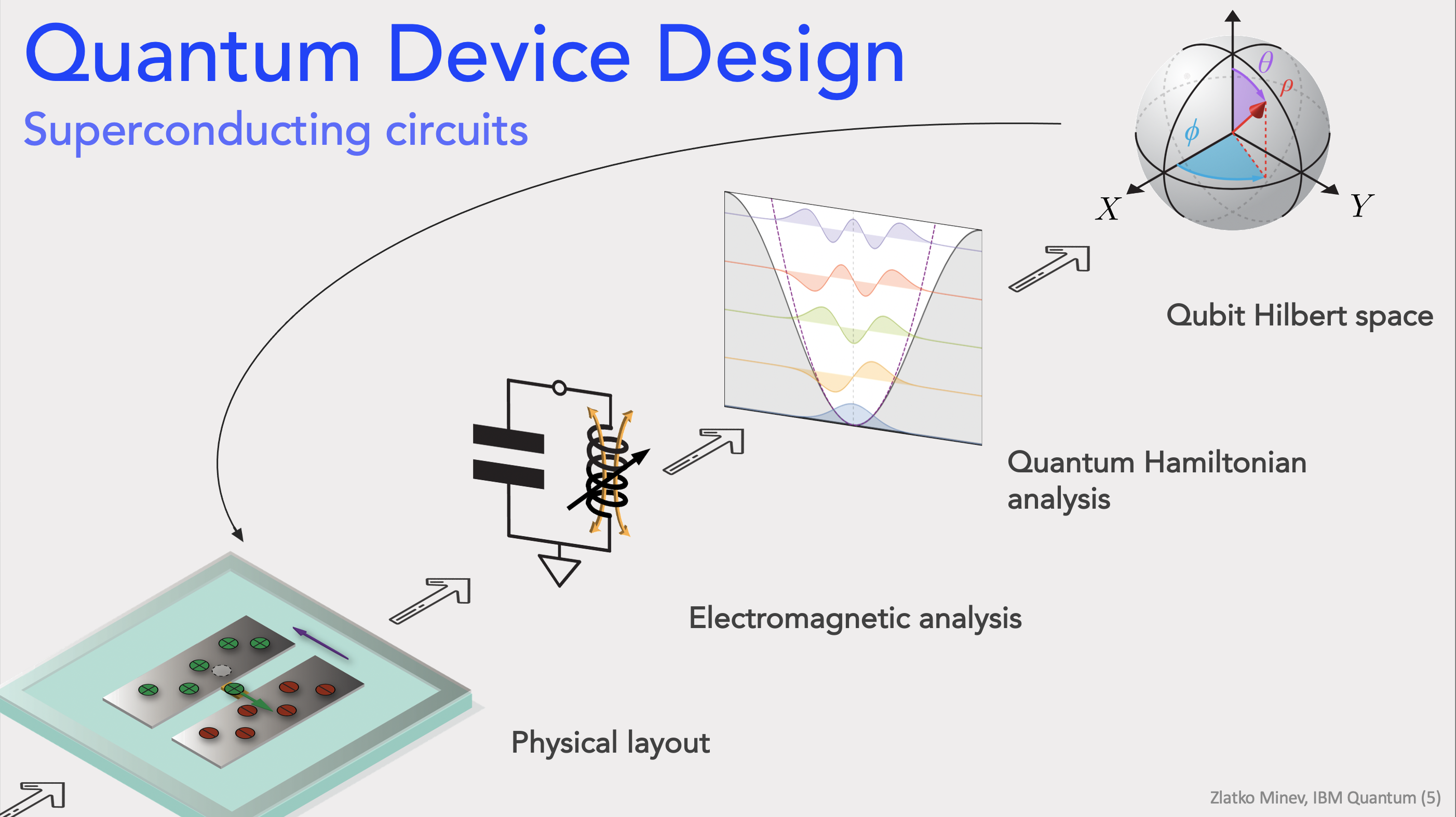
Designing quantum devices is the bedrock of the quantum ecosystem, but it is a difficult, multi-step process that connects traditionally disparate worlds. Metal is automating and streamlining this process.

Missing Workflow Diagram

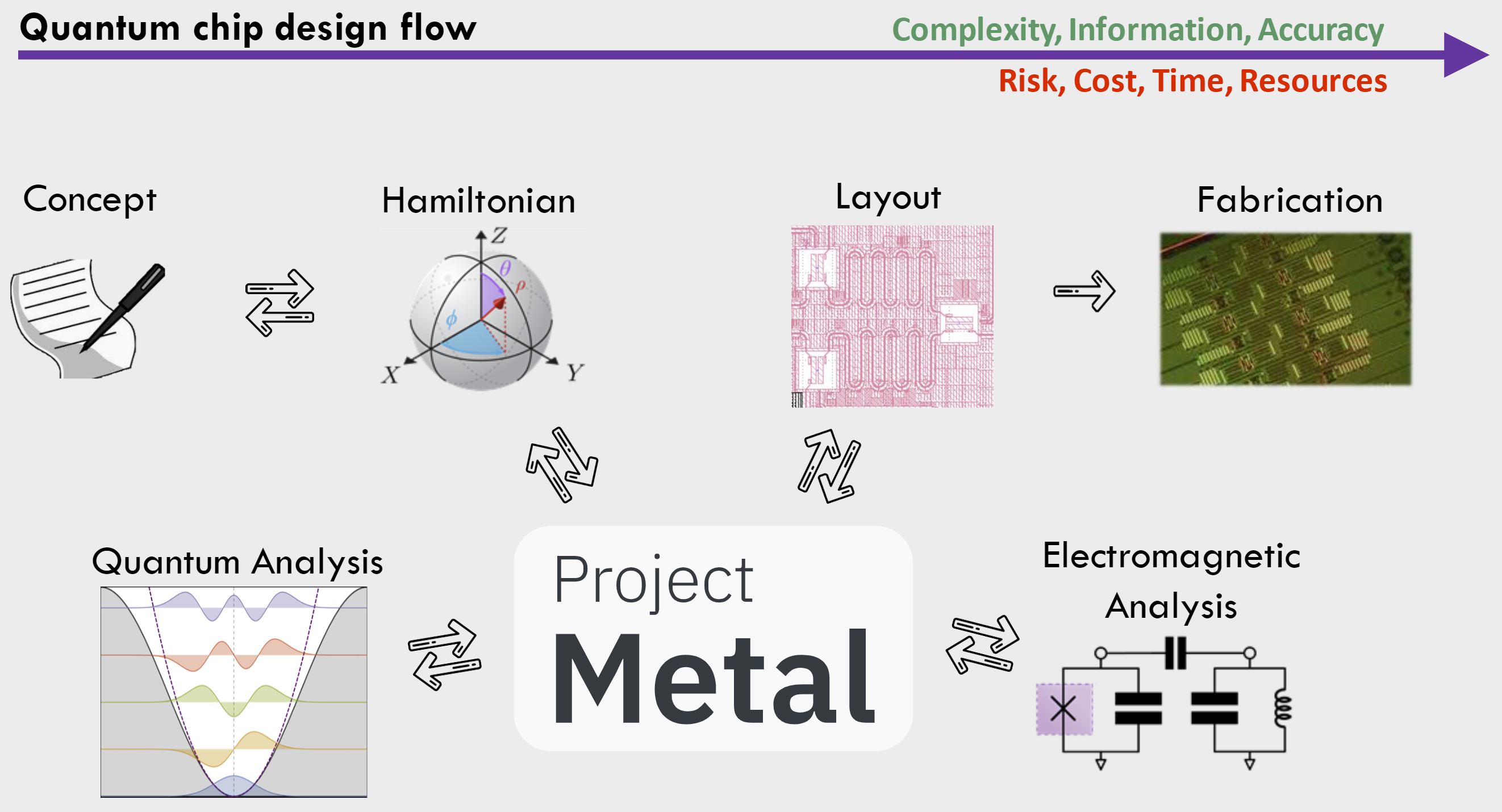
On the surface, designing a quantum chip should be a lot like designing any other integrated circuit. But a typical integrated circuit goes through a design flow process that’s had decades worth of tuning. As chips have scaled up in transistor count in step with Moore’s law, design tools have matured in kind, becoming automated. Today, a sequence of programs allow chip designers to think in a modular way about integrated circuits with billions of transistors, in a process that rather seamlessly creates and tests designs, then moves them to the fabrication stage. Quantum computers are not like today’s computer microprocessors, though. Quantum bits are much larger than transistors, and require more complex superconducting circuitry. Computer-aided electronic design automation software covers only some parts of this intricate fabrication process, and using these software packages to design a quantum computer comes with a high barrier to entry. In terms of a high-level description, we aim to perform the following tight feedback loop of design. (read the full Medium blog)

Missing Image


Quantization Methods Overview

We currently support two complementary quantization approaches that cover most day-to-day chip design work: a lightweight lumped/ quasi-lumped model and a full-wave, black-box style energy-participation ratio (EPR) workflow. Use this section as a quick “why and when” guide before you pick a solver.

What you give us - Your device geometry (from the QComponent library or your own components) - A small set of materials/stack assumptions (dielectrics, metal films, boundaries) - The excitation/ports you care about (for scattering or eigenmode solves)

What you get back - Modal frequencies, anharmonicities, and dispersive shifts - Coupling strengths and participation matrices you can plug into Hamiltonians - Loss estimates tied to specific volumes (dielectrics, conductors, seams) so you can chase the right bottleneck

Each method balances speed, fidelity, and required setup. Start with the lumped model when you need fast iteration and intuitive circuit pictures; switch to EPR when geometry and field participation really matter.

Missing Image

Lumped-oscillator model

In the lumped-oscillator model you treat each component as a compact circuit element whose capacitance and inductance can be extracted from fast quasi-static simulations or closed-form formulas. Think of it as a guided way to draw a circuit, pull out the C and L values, and then stitch those into a Hamiltonian.

When to use it. Early design and parameter sweeps when you want intuition and speed. Routing, connector placement, and first-order coupling strengths are often “good enough” here. Because solves are cheap, you can explore a lot of geometry/stack variants before moving to heavier solvers.

How it works. Partition the device into a handful of cells, solve each one quickly to get effective C/L values, then assemble the network and quantize. The reduction step preserves the pairwise couplings so you keep track of renormalization and loading. The result is a simple Hamiltonian with parameters you can iterate on in minutes.

References:

  • Zlatko K. Minev, Thomas G. McConkey, Maika Takita, Antonio Corcoles, Jay M. Gambetta, Circuit quantum electrodynamics (cQED) with modular quasi-lumped models. (2021)

Missing Image Missing Image

Energy: The energy-participation-ratio (EPR) method

The energy-participation-ratio (EPR) method is a general (black-box) quantization method. Based on the Quantum Metal integration with pyEPR, one can automate the design and quantization of Josephson quantum circuits, and even 3D circuits.

The EPR method is based on the energy-participation ratio (EPR) of a dissipative or nonlinear element in an electromagnetic mode. The EPR, a number between zero and one, quantifies how much of the energy of a mode is stored in each element. It obeys universal constraints—valid regardless of the circuit topology and nature of the nonlinear elements. The EPR of the elements are calculated from a unique, efficient electromagnetic eigenmode simulation of the linearized circuit, including lossy elements. Their set is the key input to the determination of the quantum Hamiltonian of the system. The method provides an intuitive and simple-to-use tool to quantize multi-junction circuits. It is especially well-suited for finding the Hamiltonian and dissipative parameters of weakly anharmonic systems, such as transmon qubits coupled to resonators, or Josephson transmission lines. The EPR method is experimentally tested on a variety of Josephson circuits, and demonstrated high agreement for nonlinear couplings and modal Hamiltonian parameters, over many order of magnitude in energy.

When to use it. When layout details matter: packaging effects, higher-mode participation, junction placement, seams, or substrate losses. EPR gives you a field-aware Hamiltonian and ties every loss number to a physical volume, so you know which lever to pull next.

What you set up. Draw your design, define materials and boundaries, place ports, and run a single eigenmode solve on the linearized circuit. pyEPR reads the fields, computes participations for every nonlinear/lossy element, and hands back frequencies, dispersive shifts, anharmonicities, and loss budgets. Because it is black-box, it scales to multi-mode, multi-junction systems with minimal hand-tuning.

References:

Impedance: impedance-based black-box quantization (BBQ)

The impedance formulation of black-box quantization builds the Hamiltonian directly from the frequency-dependent impedance seen between nonlinear elements and ground. It shares the “full-wave fields first, circuit later” philosophy of EPR, but works in the impedance domain: from a port-defined impedance matrix you extract effective mode frequencies, participation factors, and couplings.

When to use it. For strongly multi-port/multi-mode layouts where port impedances are the most natural handle (e.g., rich bus networks, Purcell filters, or chip-package assemblies). It is also a good cross check to EPR when you want to validate couplings via an independent pipeline.

What you set up. Define ports at the locations of junctions or pins, run an eigenmode or driven solve to obtain the impedance matrix versus frequency, then sample around the modes of interest. The resulting impedances map to effective inductive/capacitive participations and give you the Hamiltonian parameters.

Outputs. Mode frequencies, nonlinear participation, and cross-Kerr rates derived from the impedance matrix, plus a clear picture of how design changes move those impedances. Use it to tune Purcell filters, set coupling windows, or debug unexpected mode crowding.

Missing Image