Note
This page was generated from circuit-examples/full-design-flow-examples/A.4-Full-chip-design.ipynb.
A.4 Full chip design


💡 Running in Colab or Binder? Skip the desktop GUI install — the cell below grabs the lite (no-Qt) wheel, and
qm.gui(design)auto-picks an inline matplotlib viewer with the same API as the desktopMetalGUI.
🧭 Other simulation pathways. This notebook uses Ansys and ElmerFEM side by side. A third route is the pip-installable gmsh + scikit-fem solver for eigenmodes, couplings and capacitance (tutorials 4.43–4.45); AWS Palace is available through SQDMetal, with a native integration in progress. Simulation pathways summarizes what each solver computes, how to install it, and which tutorials use it.
[1]:
# In Colab / Binder, uncomment to install Quantum Metal (lite, no Qt).
# Locally you should already have it via `pip install quantum-metal` or
# `pip install 'quantum-metal[gui]'` for the desktop GUI.
# !pip install -q quantum-metal
# For the gmsh / ElmerFEM section, also:
# Colab only (not needed locally): gmsh's Linux wheel needs system graphics libraries Colab lacks.
# !apt-get -qq update && apt-get -qq install -y libglu1-mesa libgl1 libxcursor1 libxft2 libxinerama1 libxfixes3 libxrender1 libxext6 libfontconfig1 > /dev/null
# !pip install -q "quantum-metal[mesh]"
💡 Desktop GUI or inline.
metal.gui(design)opens the desktopMetalGUIwhen Qt and a display are available and falls back to an inline viewer (Colab, Binder, a server) with the same API, sogui.rebuild()andgui.screenshot()work in both. See 1.1 Quick start and`docs/headless-usage.rst<https://qiskit-community.github.io/qiskit-metal/headless-usage.html>`__.The analysis sections use Ansys (Q3D and HFSS); their outputs are from a run with Ansys installed. The layout and the GDS export run anywhere.
[2]:
import qiskit_metal as metal
from qiskit_metal import Dict, designs, draw, open_docs

%metal_heading Welcome to Qiskit Metal!
Welcome to Qiskit Metal!
This notebook builds a complete multi-qubit chip from start to finish: lay it out, analyze and tune it, and export it to GDS for fabrication.
The chip mixes the parts a real design uses: transmon pockets and crossmons with flux lines, a tunable coupler, meandered and straight transmission lines, capacitive couplers, a multiplexed readout line, and launchpads for the wire bonds. It is a teaching layout rather than a working device – the resonator lengths are only roughly chosen – but every step is the one you would take on a real chip.
What you’ll do
Layout – place the qubits, connect them with buses, add readout and control lines.
Analyze – extract the capacitance matrix and run the lumped-oscillator model (LOM) with Ansys Q3D, then an eigenmode simulation and energy-participation (EPR) analysis with HFSS.
Export – write the mask to GDS.
Layout
[3]:
from qiskit_metal.qlibrary.qubits.transmon_pocket_6 import TransmonPocket6
from qiskit_metal.qlibrary.qubits.transmon_cross_fl import TransmonCrossFL

from qiskit_metal.qlibrary.couplers.tunable_coupler_01 import TunableCoupler01

from qiskit_metal.qlibrary.tlines.meandered import RouteMeander
from qiskit_metal.qlibrary.tlines.pathfinder import RoutePathfinder
from qiskit_metal.qlibrary.tlines.anchored_path import RouteAnchors

from qiskit_metal.qlibrary.lumped.cap_n_interdigital import CapNInterdigital
from qiskit_metal.qlibrary.couplers.cap_n_interdigital_tee import CapNInterdigitalTee
from qiskit_metal.qlibrary.couplers.coupled_line_tee import CoupledLineTee

from qiskit_metal.qlibrary.terminations.launchpad_wb import LaunchpadWirebond
from qiskit_metal.qlibrary.terminations.launchpad_wb_coupled import (
    LaunchpadWirebondCoupled,
)
[4]:
design = metal.designs.DesignPlanar()

gui = metal.gui(design)
qm.view(design); gui.rebuild(), gui.screenshot(), gui.edit_component(...) work as in the desktop GUI.For the full desktop experience (Qt window, dockable panels):
pip install 'quantum-metal[gui]' and re-import.Since we are likely to be making many changes while tuning and modifying our design, we will enable overwriting. We can also check all of the chip properties to see if we want to change the size or any other parameter.
[5]:
design.overwrite_enabled = True
design.chips.main
[5]:
{'material': 'silicon',
 'layer_start': '0',
 'layer_end': '2048',
 'size': {'center_x': '0.0mm',
  'center_y': '0.0mm',
  'center_z': '0.0mm',
  'size_x': '9mm',
  'size_y': '6mm',
  'size_z': '-750um',
  'sample_holder_top': '890um',
  'sample_holder_bottom': '1650um'}}
[6]:
# 11 mm x 8 mm, centered 0.5 mm below the origin so the launchpads sit at the
# chip edges.
design.chips.main.size.size_x = "11mm"
design.chips.main.size.size_y = "8mm"
design.chips.main.size.center_y = "-0.5mm"
The Qubits
We will add a collection of qubits. First we will place a transmon pocket with six connection pads. We can see any options the qubit qcomponent has to figure out what we might want to modify when creating the component. This will include the components default options (which the component designer included) as well as renderer options (which are added based on what renderers are present in Metal).
[7]:
TransmonPocket6.get_template_options(design)
[7]:
{'pos_x': '0.0um',
 'pos_y': '0.0um',
 'orientation': '0.0',
 'chip': 'main',
 'layer': '1',
 'connection_pads': {},
 '_default_connection_pads': {'pad_gap': '15um',
  'pad_width': '125um',
  'pad_height': '30um',
  'pad_cpw_shift': '0um',
  'pad_cpw_extent': '25um',
  'cpw_width': '10um',
  'cpw_gap': '6um',
  'cpw_extend': '100um',
  'pocket_extent': '5um',
  'pocket_rise': '0um',
  'loc_W': '+1',
  'loc_H': '+1'},
 'pad_gap': '30um',
 'inductor_width': '20um',
 'pad_width': '455um',
 'pad_height': '90um',
 'pocket_width': '650um',
 'pocket_height': '650um',
 'hfss_wire_bonds': False,
 'q3d_wire_bonds': False,
 'aedt_q3d_wire_bonds': False,
 'aedt_hfss_wire_bonds': False,
 'hfss_inductance': '10nH',
 'hfss_capacitance': 0,
 'hfss_resistance': 0,
 'hfss_mesh_kw_jj': 7e-06,
 'q3d_inductance': '10nH',
 'q3d_capacitance': 0,
 'q3d_resistance': 0,
 'q3d_mesh_kw_jj': 7e-06,
 'gds_cell_name': 'my_other_junction',
 'aedt_q3d_inductance': 1e-08,
 'aedt_q3d_capacitance': 0,
 'aedt_hfss_inductance': 1e-08,
 'aedt_hfss_capacitance': 0}
[8]:
options = dict(
    pad_width="425 um",
    pocket_height="650um",
    connection_pads=dict(
        readout=dict(loc_W=0, loc_H=-1, pad_width="80um", pad_gap="50um"),
        bus_01=dict(loc_W=-1, loc_H=-1, pad_width="60um", pad_gap="10um"),
        bus_02=dict(loc_W=-1, loc_H=+1, pad_width="60um", pad_gap="10um"),
        bus_03=dict(loc_W=0, loc_H=+1, pad_width="90um", pad_gap="30um"),
        bus_04=dict(loc_W=+1, loc_H=+1, pad_width="60um", pad_gap="10um"),
        bus_05=dict(loc_W=+1, loc_H=-1, pad_width="60um", pad_gap="10um"),
    ),
)

q_main = TransmonPocket6(
    design,
    "Q_Main",
    options=dict(
        pos_x="0mm",
        pos_y="-1mm",
        gds_cell_name="FakeJunction_01",
        hfss_inductance="14nH",
        **options,
    ),
)

gui.rebuild()
gui.autoscale()
[8]:
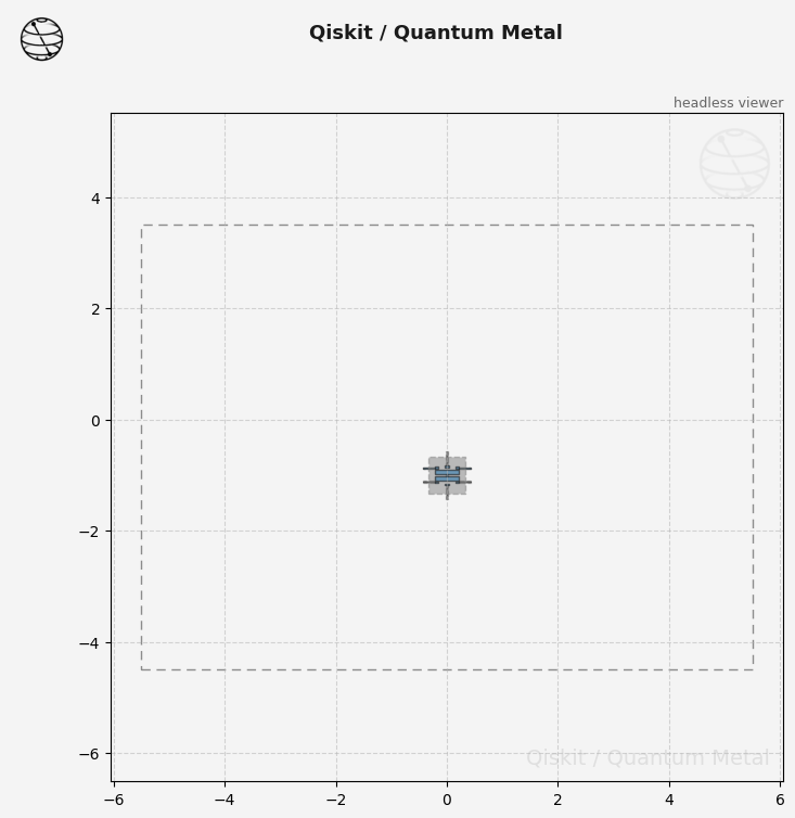
We then will add a mixture of additional qubits. This is not (though do not let me stop any experimental investigation) a design one would normally create for any experiment of computational purpose, but allows for having a mixture of different components on one chip.
[9]:
TransmonCrossFL.get_template_options(design)
[9]:
{'pos_x': '0.0um',
 'pos_y': '0.0um',
 'orientation': '0.0',
 'chip': 'main',
 'layer': '1',
 'connection_pads': {},
 '_default_connection_pads': {'connector_type': '0',
  'claw_length': '30um',
  'ground_spacing': '5um',
  'ground_spacing_back': None,
  'claw_width': '10um',
  'claw_width_back': None,
  'claw_gap': '6um',
  'claw_cpw_length': '40um',
  'claw_cpw_width': '10um',
  'connector_location': '0'},
 'cross_width': '20um',
 'cross_length': '200um',
 'cross_gap': '20um',
 'make_fl': True,
 'fl_options': {'t_top': '15um',
  't_offset': '0um',
  't_inductive_gap': '3um',
  't_width': '5um',
  't_gap': '3um'},
 'hfss_wire_bonds': False,
 'q3d_wire_bonds': False,
 'aedt_q3d_wire_bonds': False,
 'aedt_hfss_wire_bonds': False,
 'hfss_inductance': '10nH',
 'hfss_capacitance': 0,
 'hfss_resistance': 0,
 'hfss_mesh_kw_jj': 7e-06,
 'q3d_inductance': '10nH',
 'q3d_capacitance': 0,
 'q3d_resistance': 0,
 'q3d_mesh_kw_jj': 7e-06,
 'gds_cell_name': 'my_other_junction',
 'aedt_q3d_inductance': 1e-08,
 'aedt_q3d_capacitance': 0,
 'aedt_hfss_inductance': 1e-08,
 'aedt_hfss_capacitance': 0}
We will add two crossmons with flux lines to the west side of the chip, which we will couple to each other using a tunable coupler. To make sure the various readout and control lines will have space to connect to launchers at the chip edge, we have to be mindful of where we place them, and making sure we have enough space for routing while avoiding cross talk.
[10]:
Q1 = TransmonCrossFL(
    design,
    "Q1",
    options=dict(
        pos_x="-2.75mm",
        pos_y="-1.8mm",
        connection_pads=dict(
            bus_01=dict(connector_location="180", claw_length="95um"),
            readout=dict(connector_location="0"),
        ),
        fl_options=dict(),
    ),
)

Q2 = TransmonCrossFL(
    design,
    "Q2",
    options=dict(
        pos_x="-2.75mm",
        pos_y="-1.2mm",
        orientation="180",
        connection_pads=dict(
            bus_02=dict(connector_location="0", claw_length="95um"),
            readout=dict(connector_location="180"),
        ),
        fl_options=dict(),
    ),
)


tune_c_Q12 = TunableCoupler01(
    design,
    "Tune_C_Q12",
    options=dict(pos_x="-2.81mm", pos_y="-1.5mm", orientation=90, c_width="500um"),
)

gui.rebuild()
gui.autoscale()
[10]:
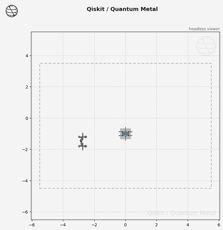
We then will add three transmon pockets to the north side of the chip, with the intention of having them in a linear series of coupling to each other, as well as the ‘main’ qubit to the south.
[11]:
Q3 = TransmonPocket6(
    design,
    "Q3",
    options=dict(
        pos_x="-3mm",
        pos_y="0.5mm",
        gds_cell_name="FakeJunction_01",
        hfss_inductance="14nH",
        connection_pads=dict(
            bus_03=dict(loc_W=0, loc_H=-1, pad_width="80um", pad_gap="15um"),
            bus_q3_q4=dict(loc_W=1, loc_H=-1, pad_width="80um", pad_gap="15um"),
            readout=dict(loc_W=0, loc_H=1, pad_width="80um", pad_gap="50um"),
        ),
    ),
)

Q4 = TransmonPocket6(
    design,
    "Q4",
    options=dict(
        pos_x="0mm",
        pos_y="1mm",
        gds_cell_name="FakeJunction_01",
        hfss_inductance="14nH",
        connection_pads=dict(
            bus_04=dict(loc_W=0, loc_H=-1, pad_width="80um", pad_gap="15um"),
            bus_q3_q4=dict(loc_W=-1, loc_H=-1, pad_width="80um", pad_gap="15um"),
            bus_q4_q5=dict(loc_W=1, loc_H=-1, pad_width="80um", pad_gap="15um"),
            readout=dict(loc_W=0, loc_H=1, pad_width="80um", pad_gap="50um"),
        ),
    ),
)

Q5 = TransmonPocket6(
    design,
    "Q5",
    options=dict(
        pos_x="3mm",
        pos_y="0.5mm",
        gds_cell_name="FakeJunction_01",
        hfss_inductance="14nH",
        connection_pads=dict(
            bus_05=dict(loc_W=0, loc_H=-1, pad_width="80um", pad_gap="15um"),
            bus_q4_q5=dict(loc_W=-1, loc_H=-1, pad_width="80um", pad_gap="15um"),
            readout=dict(loc_W=0, loc_H=1, pad_width="80um", pad_gap="50um"),
        ),
    ),
)
The Busses
We now couple the qubits to each other, primarily using RouteMeander. Although one needs to run simulations to properly tune the line lengths for target frequencies, an initial estimate could be determined from the below method;
[12]:
from qiskit_metal.analyses.em.cpw_calculations import guided_wavelength


def find_resonator_length(frequency, line_width, line_gap, N):
    # frequency in GHz
    # line_width/line_gap in um
    # N -> 2 for lambda/2, 4 for lambda/4

    [lambdaG, etfSqrt, q] = guided_wavelength(
        frequency * 10**9,
        line_width * 10**-6,
        line_gap * 10**-6,
        750 * 10**-6,
        200 * 10**-9,
    )
    return str(lambdaG / N * 10**3) + " mm"
As we are not worried about creating a functional chip in this tutorial, we will give the resonators somewhat arbitrary lengths. First coupling the two crossmons to Q_Main.
[13]:
bus_01 = RouteMeander(
    design,
    "Bus_01",
    options=dict(
        hfss_wire_bonds=True,
        pin_inputs=Dict(
            start_pin=Dict(component="Q_Main", pin="bus_01"),
            end_pin=Dict(component="Q1", pin="bus_01"),
        ),
        lead=Dict(start_straight="125um", end_straight="225um"),
        meander=Dict(asymmetry="1305um", spacing="250um"),
        fillet="99um",
        total_length="6mm",
    ),
)

bus_02 = RouteMeander(
    design,
    "Bus_02",
    options=dict(
        hfss_wire_bonds=True,
        pin_inputs=Dict(
            start_pin=Dict(component="Q_Main", pin="bus_02"),
            end_pin=Dict(component="Q2", pin="bus_02"),
        ),
        lead=Dict(start_straight="325um", end_straight="125um"),
        meander=Dict(asymmetry="450um"),
        fillet="99um",
        total_length="6.4mm",
    ),
)


gui.rebuild()
[13]:
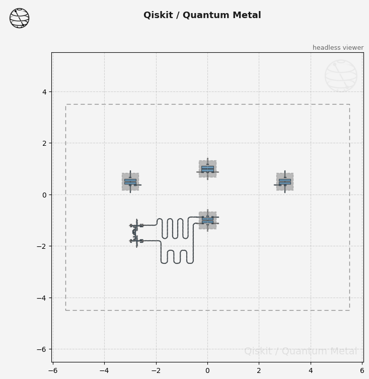
Then the three transmon pockets on the north side to Q_Main.
[14]:
bus_03 = RouteMeander(
    design,
    "Bus_03",
    options=dict(
        hfss_wire_bonds=True,
        pin_inputs=Dict(
            start_pin=Dict(component="Q_Main", pin="bus_03"),
            end_pin=Dict(component="Q3", pin="bus_03"),
        ),
        lead=Dict(start_straight="225um", end_straight="25um"),
        meander=Dict(asymmetry="50um"),
        fillet="99um",
        total_length="6.8mm",
    ),
)

# To help set the right spacing, jogs can be used to set some initially controlled routing paths
from collections import OrderedDict

jogs_start = OrderedDict()
jogs_start[0] = ["L", "250um"]
jogs_start[1] = ["R", "200um"]

jogs_end = OrderedDict()
jogs_end[0] = ["L", "600um"]

bus_04 = RouteMeander(
    design,
    "Bus_04",
    options=dict(
        hfss_wire_bonds=True,
        pin_inputs=Dict(
            start_pin=Dict(component="Q_Main", pin="bus_04"),
            end_pin=Dict(component="Q4", pin="bus_04"),
        ),
        lead=Dict(
            start_straight="225um",
            # end_straight = '25um',
            start_jogged_extension=jogs_start,
            # end_jogged_extension = jogs_end
        ),
        meander=Dict(asymmetry="150um"),
        fillet="99um",
        total_length="7.2mm",
    ),
)

bus_05 = RouteMeander(
    design,
    "Bus_05",
    options=dict(
        hfss_wire_bonds=True,
        pin_inputs=Dict(
            start_pin=Dict(component="Q_Main", pin="bus_05"),
            end_pin=Dict(component="Q5", pin="bus_05"),
        ),
        lead=Dict(start_straight="225um", end_straight="25um"),
        meander=Dict(asymmetry="50um"),
        fillet="99um",
        total_length="7.6mm",
    ),
)

gui.rebuild()
[14]:
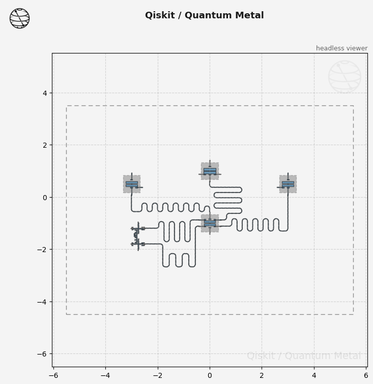
Finally the three transmon pockets on the north side to each other. This concludes the interconnectivity between the qubits.
[15]:
bus_q3_q4 = RouteMeander(
    design,
    "Bus_Q3_Q4",
    options=dict(
        hfss_wire_bonds=True,
        pin_inputs=Dict(
            start_pin=Dict(component="Q3", pin="bus_q3_q4"),
            end_pin=Dict(component="Q4", pin="bus_q3_q4"),
        ),
        lead=Dict(start_straight="125um", end_straight="125um"),
        meander=Dict(asymmetry="50um"),
        fillet="99um",
        total_length="6.4mm",
    ),
)

bus_q4_q5 = RouteMeander(
    design,
    "Bus_Q4_Q5",
    options=dict(
        hfss_wire_bonds=True,
        pin_inputs=Dict(
            start_pin=Dict(component="Q4", pin="bus_q4_q5"),
            end_pin=Dict(component="Q5", pin="bus_q4_q5"),
        ),
        lead=Dict(start_straight="125um", end_straight="25um"),
        meander=Dict(asymmetry="50um"),
        fillet="99um",
        total_length="6.8mm",
    ),
)

gui.rebuild()
[15]:
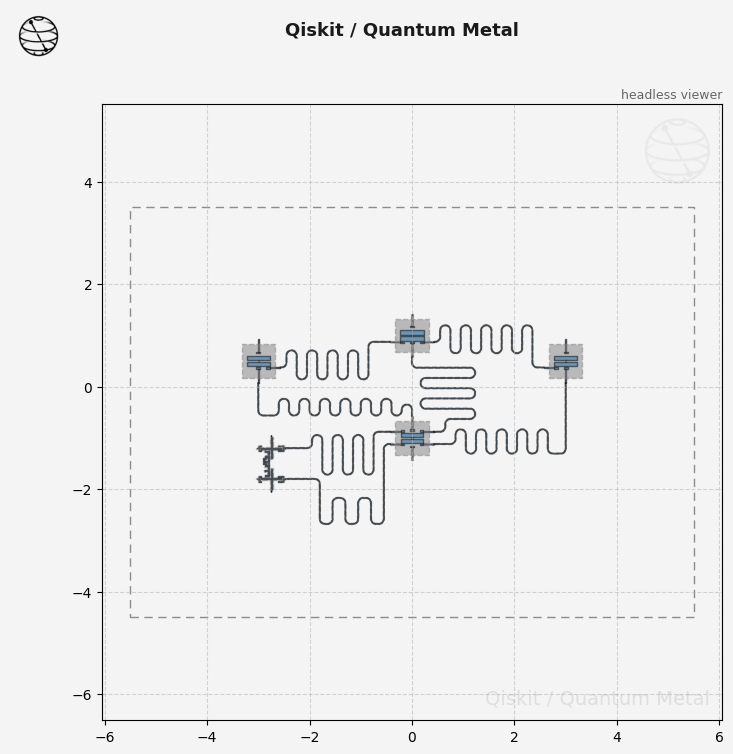
The Readouts and Control Lines
The intention for this design is to have the three north transmon pockets be multiplexed to one readout line. The crossmons to their own readouts, as well as Q_Main. The tunable coupler, and the two crossmons also have flux lines which need to be connected to launchers. First we will place the wirebond launchers at the edges of the chip.
[16]:
launch_qmain_read = LaunchpadWirebond(
    design,
    "Launch_QMain_Read",
    options=dict(pos_x="2mm", pos_y="-4mm", orientation="90"),
)

launch_q1_fl = LaunchpadWirebond(
    design,
    "Launch_Q1_FL",
    options=dict(
        pos_x="0mm",
        pos_y="-4mm",
        orientation="90",
        trace_width="5um",
        trace_gap="3um",
    ),
)
launch_q1_read = LaunchpadWirebondCoupled(
    design, "Launch_Q1_Read", options=dict(pos_x="-2mm", pos_y="-4mm", orientation="90")
)

launch_tcoup_fl = LaunchpadWirebond(
    design,
    "Launch_TuneC_FL",
    options=dict(
        pos_x="-4mm",
        pos_y="-4mm",
        orientation="90",
        trace_width="5um",
        trace_gap="3um",
    ),
)
launch_tcoup_read = LaunchpadWirebondCoupled(
    design,
    "Launch_TuneC_Read",
    options=dict(pos_x="-5mm", pos_y="-3mm", orientation="0"),
)

launch_q2_read = LaunchpadWirebondCoupled(
    design, "Launch_Q2_Read", options=dict(pos_x="-5mm", pos_y="-1mm", orientation="0")
)
launch_q2_fl = LaunchpadWirebond(
    design,
    "Launch_Q2_FL",
    options=dict(
        pos_x="-5mm",
        pos_y="1mm",
        orientation="0",
        trace_width="5um",
        trace_gap="3um",
    ),
)

launch_nw = LaunchpadWirebond(
    design, "Launch_NW", options=dict(pos_x="-5mm", pos_y="3mm", orientation=0)
)
launch_ne = LaunchpadWirebond(
    design, "Launch_NE", options=dict(pos_x="5mm", pos_y="3mm", orientation=180)
)


gui.rebuild()
[16]:
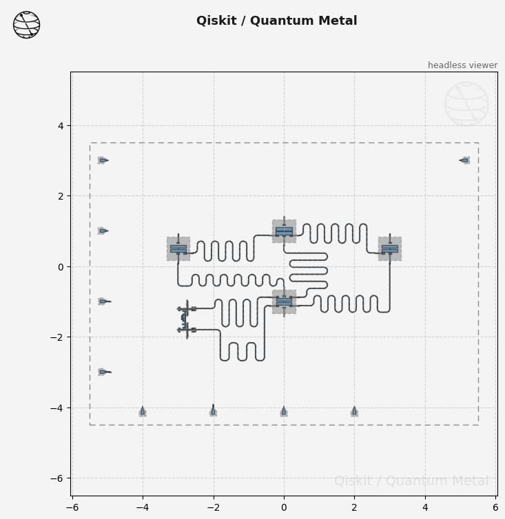
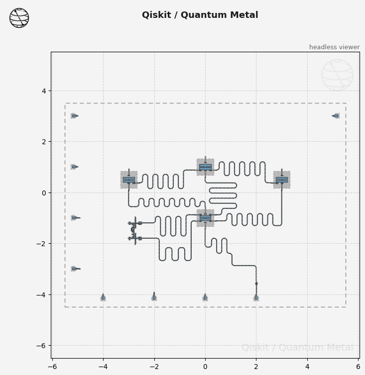
We then will add in the readout resonators for Q_Main, Q1, Q2 and the tuneable coupler. We will add a finger capacitor for the Q_Main readout, instead of just using the LaunchpadWirebondCoupled.
[17]:
# Main Readout


read_q_main_cap = CapNInterdigital(
    design,
    "Read_Q_Main_Cap",
    options=dict(pos_x="2mm", pos_y="-3.5mm", orientation="0"),
)

jogs_end = OrderedDict()
jogs_end[0] = ["L", "600um"]

jogs_start = OrderedDict()
jogs_start[0] = ["L", "250um"]

read_q_main = RouteMeander(
    design,
    "Read_Q_Main",
    options=dict(
        hfss_wire_bonds=True,
        pin_inputs=Dict(
            start_pin=Dict(component="Q_Main", pin="readout"),
            end_pin=Dict(component="Read_Q_Main_Cap", pin="north_end"),
        ),
        lead=Dict(
            start_straight="725um",
            end_straight="625um",
            start_jogged_extension=jogs_start,
            end_jogged_extension=jogs_end,
        ),
        meander=Dict(asymmetry="50um"),
        fillet="99um",
        total_length="5.6mm",
    ),
)

read_q_main_cap_launch = RoutePathfinder(
    design,
    "Read_Q_Main_Cap_Launch",
    options=dict(
        hfss_wire_bonds=True,
        pin_inputs=dict(
            start_pin=Dict(component="Read_Q_Main_Cap", pin="south_end"),
            end_pin=Dict(component="Launch_QMain_Read", pin="tie"),
        ),
        lead=Dict(
            start_straight="0um",
            end_straight="0um",
            # start_jogged_extension = jogs_start,
            # end_jogged_extension = jogs_end
        ),
    ),
)


gui.rebuild()
[17]:
[18]:
# Crossmon's Readouts

jogs_end = OrderedDict()
jogs_end[0] = ["L", "600um"]

jogs_start = OrderedDict()
jogs_start[0] = ["L", "250um"]

read_q1 = RouteMeander(
    design,
    "Read_Q1",
    options=dict(
        hfss_wire_bonds=True,
        pin_inputs=Dict(
            start_pin=Dict(component="Q1", pin="readout"),
            end_pin=Dict(component="Launch_Q1_Read", pin="tie"),
        ),
        lead=Dict(
            start_straight="250um",
            end_straight="25um",
            # start_jogged_extension = jogs_start,
            # end_jogged_extension = jogs_end
        ),
        meander=Dict(asymmetry="50um"),
        fillet="99um",
        total_length="6.8mm",
    ),
)


jogs_end = OrderedDict()
jogs_end[0] = ["L", "600um"]

jogs_start = OrderedDict()
jogs_start[0] = ["L", "250um"]

read_tunec = RouteMeander(
    design,
    "Read_TuneC",
    options=dict(
        hfss_wire_bonds=True,
        pin_inputs=Dict(
            start_pin=Dict(component="Tune_C_Q12", pin="Control"),
            end_pin=Dict(component="Launch_TuneC_Read", pin="tie"),
        ),
        lead=Dict(
            start_straight="1525um",
            end_straight="125um",
            # start_jogged_extension = jogs_start,
            # end_jogged_extension = jogs_end
        ),
        meander=Dict(asymmetry="50um"),
        fillet="99um",
        total_length="5.8mm",
    ),
)

jogs_end = OrderedDict()
jogs_end[0] = ["L", "600um"]

jogs_start = OrderedDict()
jogs_start[0] = ["L", "250um"]


read_q2 = RouteMeander(
    design,
    "Read_Q2",
    options=dict(
        hfss_wire_bonds=True,
        pin_inputs=Dict(
            start_pin=Dict(component="Q2", pin="readout"),
            end_pin=Dict(component="Launch_Q2_Read", pin="tie"),
        ),
        lead=Dict(
            start_straight="350um",
            end_straight="0um",
            # start_jogged_extension = jogs_start,
            # end_jogged_extension = jogs_end
        ),
        meander=Dict(asymmetry="-450um"),
        fillet="99um",
        total_length="5.4mm",
    ),
)


gui.rebuild()
[18]:
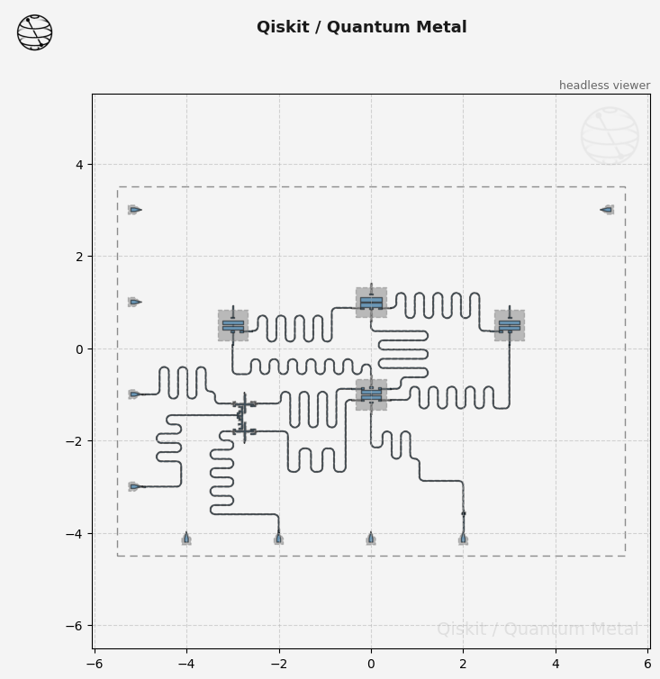
Finishing off this section of the chip by connecting the flux lines to appropraite wirebond launch pads.
[19]:
# Crossmon flux lines

flux_line_Q1 = RoutePathfinder(
    design,
    "Flux_Line_Q1",
    options=dict(
        hfss_wire_bonds=True,
        pin_inputs=Dict(
            start_pin=Dict(component="Q1", pin="flux_line"),
            end_pin=Dict(component="Launch_Q1_FL", pin="tie"),
        ),
        fillet="99um",
        trace_width="5um",
        trace_gap="3um",
        # anchors = anchors
    ),
)


jogs_start = OrderedDict()
jogs_start[0] = ["L", "750um"]

flux_line_tunec = RoutePathfinder(
    design,
    "Flux_Line_TuneC",
    options=dict(
        hfss_wire_bonds=True,
        pin_inputs=Dict(
            start_pin=Dict(component="Tune_C_Q12", pin="Flux"),
            end_pin=Dict(component="Launch_TuneC_FL", pin="tie"),
        ),
        lead=Dict(
            start_straight="875um",
            end_straight="350um",
            start_jogged_extension=jogs_start,
            # end_jogged_extension = jogs_end
        ),
        fillet="99um",
        trace_width="5um",
        trace_gap="3um",
        # anchors = anchors
    ),
)


jogs_start = OrderedDict()
jogs_start[0] = ["L", "525um"]
jogs_start[1] = ["R", "625um"]

flux_line_Q2 = RoutePathfinder(
    design,
    "Flux_Line_Q2",
    options=dict(
        hfss_wire_bonds=True,
        pin_inputs=Dict(
            start_pin=Dict(component="Q2", pin="flux_line"),
            end_pin=Dict(component="Launch_Q2_FL", pin="tie"),
        ),
        lead=Dict(
            start_straight="175um",
            end_straight="150um",
            start_jogged_extension=jogs_start,
            # end_jogged_extension = jogs_end
        ),
        fillet="99um",
        trace_width="5um",
        trace_gap="3um",
        # anchors = anchors
    ),
)

gui.rebuild()
[19]:
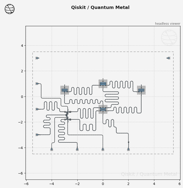
Shifting our focus now to the three transmon pockets in the north. As we want these to be multiplexed to a single readout line, we will add in a few three port components, such as the CoupledLineTee and CapNInterdigitalTee. Q3 will have an inductive coupling to the readout line (as we want a lambda/4 resonator), Q4 will have a simple gap capacitor, and Q5 will have an interdigitated capacitor.
[20]:
q3_read_T = CoupledLineTee(
    design,
    "Q3_Read_T",
    options=dict(
        pos_x="-3mm",
        pos_y="3mm",
        orientation="0",
        coupling_length="200um",
        open_termination=False,
    ),
)
# We use finger count to set the width of the gap capacitance, -> N*cap_width + (N-1)*cap_gap
q4_read_T = CapNInterdigitalTee(
    design,
    "Q4_Read_T",
    options=dict(
        pos_x="0mm", pos_y="3mm", orientation="0", finger_length="0um", finger_count="8"
    ),
)
q5_read_T = CapNInterdigitalTee(
    design,
    "Q5_Read_T",
    options=dict(
        pos_x="3mm",
        pos_y="3mm",
        orientation="0",
        finger_length="50um",
        finger_count="11",
    ),
)

gui.rebuild()
[20]:
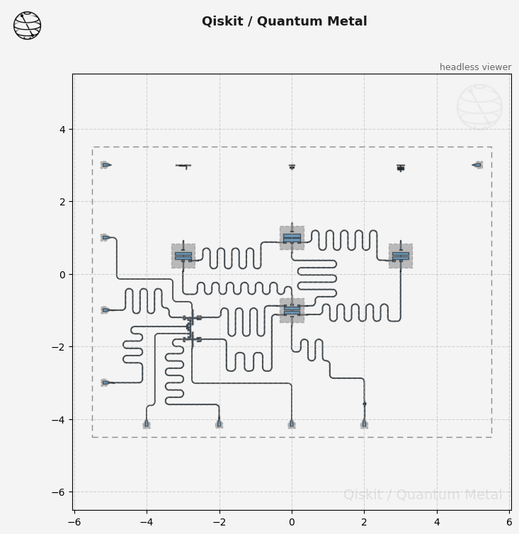
We add in the readout resonators to each respective qubit.
[21]:
read_q3 = RouteMeander(
    design,
    "Read_Q3",
    options=dict(
        hfss_wire_bonds=True,
        pin_inputs=Dict(
            start_pin=Dict(component="Q3", pin="readout"),
            end_pin=Dict(component="Q3_Read_T", pin="second_end"),
        ),
        lead=Dict(
            start_straight="150um",
            end_straight="150um",
            # start_jogged_extension = jogs_start,
            # end_jogged_extension = jogs_end
        ),
        meander=Dict(asymmetry="0um"),
        fillet="99um",
        total_length="5mm",
    ),
)

read_q4 = RouteMeander(
    design,
    "Read_Q4",
    options=dict(
        hfss_wire_bonds=True,
        pin_inputs=Dict(
            start_pin=Dict(component="Q4", pin="readout"),
            end_pin=Dict(component="Q4_Read_T", pin="second_end"),
        ),
        lead=Dict(
            start_straight="125um",
            end_straight="125um",
            # start_jogged_extension = jogs_start,
            # end_jogged_extension = jogs_end
        ),
        meander=Dict(asymmetry="0um"),
        fillet="99um",
        total_length="5.8mm",
    ),
)

read_q5 = RouteMeander(
    design,
    "Read_Q5",
    options=dict(
        hfss_wire_bonds=True,
        pin_inputs=Dict(
            start_pin=Dict(component="Q5", pin="readout"),
            end_pin=Dict(component="Q5_Read_T", pin="second_end"),
        ),
        lead=Dict(
            start_straight="125um",
            end_straight="125um",
            # start_jogged_extension = jogs_start,
            # end_jogged_extension = jogs_end
        ),
        meander=Dict(asymmetry="0um"),
        fillet="99um",
        total_length="5.4mm",
    ),
)

gui.rebuild()
[21]:
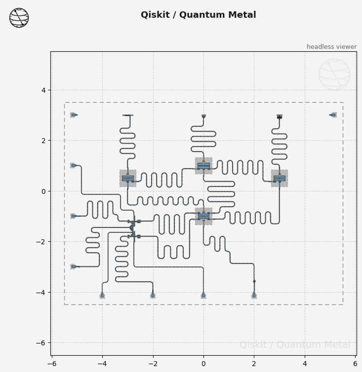
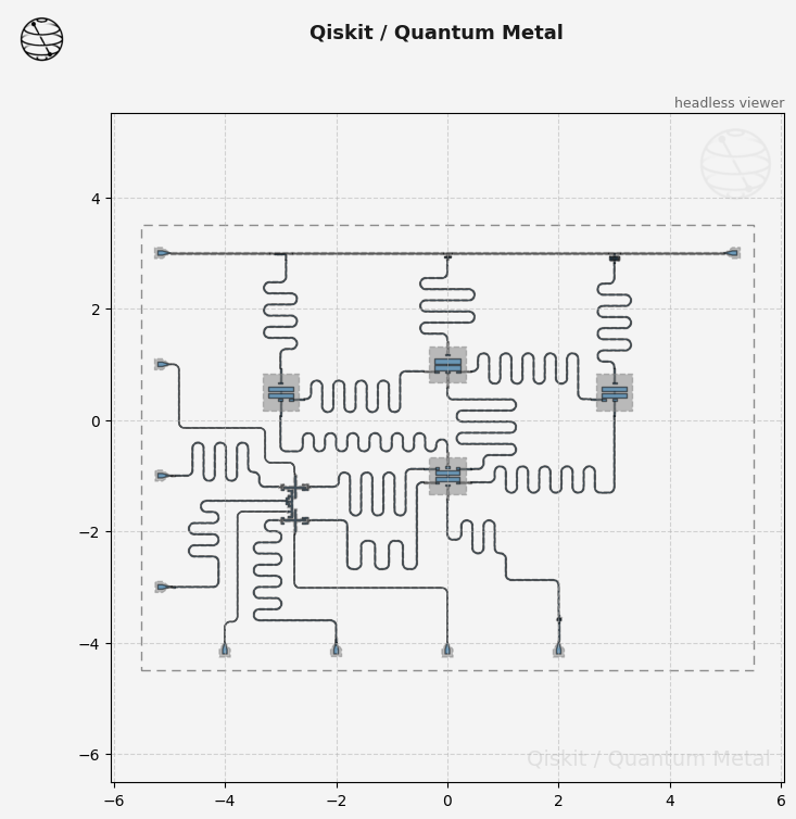
We complete the layout by connecting the multiplexed readout line to the launchpads on either side of the chip.
[22]:
mp_tl_01 = RoutePathfinder(
    design,
    "ML_TL_01",
    options=dict(
        hfss_wire_bonds=True,
        pin_inputs=dict(
            start_pin=Dict(component="Launch_NW", pin="tie"),
            end_pin=Dict(component="Q3_Read_T", pin="prime_start"),
        ),
    ),
)

mp_tl_02 = RoutePathfinder(
    design,
    "ML_TL_02",
    options=dict(
        hfss_wire_bonds=True,
        pin_inputs=dict(
            start_pin=Dict(component="Q3_Read_T", pin="prime_end"),
            end_pin=Dict(component="Q4_Read_T", pin="prime_start"),
        ),
    ),
)

mp_tl_03 = RoutePathfinder(
    design,
    "ML_TL_03",
    options=dict(
        hfss_wire_bonds=True,
        pin_inputs=dict(
            start_pin=Dict(component="Q4_Read_T", pin="prime_end"),
            end_pin=Dict(component="Q5_Read_T", pin="prime_start"),
        ),
    ),
)

mp_tl_04 = RoutePathfinder(
    design,
    "ML_TL_04",
    options=dict(
        hfss_wire_bonds=True,
        pin_inputs=dict(
            start_pin=Dict(component="Q5_Read_T", pin="prime_end"),
            end_pin=Dict(component="Launch_NE", pin="tie"),
        ),
    ),
)

gui.rebuild()
[22]:
[23]:
# Rebuild the design in the GUI and save a screenshot as a .png file.

gui.rebuild()
gui.autoscale()
gui.screenshot()
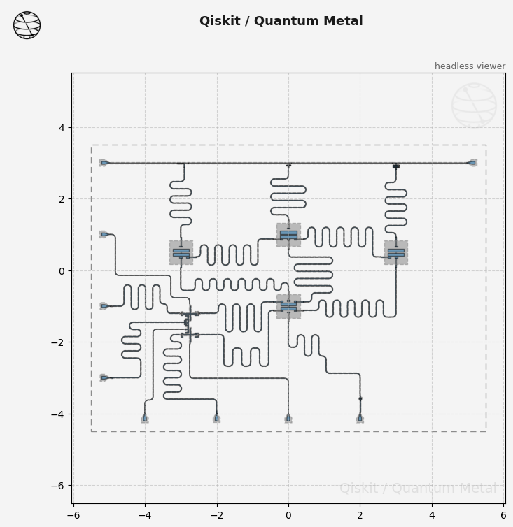
With this, the layout is complete.
Anyone familiar with chip design will spot choices a real chip would revisit – a few transmission lines run closer to each other than you would want for crosstalk, and some of the chip is unused. Compacting the layout means moving components and rerouting, which the same code makes easy to iterate on. For this tutorial, we move on to analysis and tuning.
Analyze
Capacitance Extraction and LOM
First we want to quickly look at the qubit parameters. Initial simulation and analysis is to use a lumped element approximation, by extracting the capacitance matrix of the qubit. We first analyze the qubit Q_Main, by first extracting the matrix and then using LOM analysis on it.
For starters, let’s select the appropriate QAnalysis class.
[ ]:
from qiskit_metal.analyses.quantization import LOManalysis

c1 = LOManalysis(design, "q3d")
We can check if we wish to change any of the default options for the analysis. You should modify the number of passes and convergence based on the accuracy you require for your simulation.
Depending on the complexity of the simulation, it could take a minute, or multiple hours. It is generally best to start with a small number of max_passes if you are unsure, so can you get a sense on the timing. As each adaptive pass adds additional tetrahedrons, the simulation time per pass will increase significantly (as well as the amount of system memory necessary).
[25]:
c1.sim.setup
[25]:
{'name': 'Setup',
 'reuse_selected_design': True,
 'freq_ghz': 5.0,
 'save_fields': False,
 'enabled': True,
 'max_passes': 15,
 'min_passes': 2,
 'min_converged_passes': 2,
 'percent_error': 0.5,
 'percent_refinement': 30,
 'auto_increase_solution_order': True,
 'solution_order': 'High',
 'solver_type': 'Iterative'}
[26]:
c1.sim.setup.name = "Tune_Q_Main"
c1.sim.setup.max_passes = 16
c1.sim.setup.min_converged_passes = 2
c1.sim.setup.percent_error = 0.05
c1.sim.setup
[26]:
{'name': 'Tune_Q_Main',
 'reuse_selected_design': True,
 'freq_ghz': 5.0,
 'save_fields': False,
 'enabled': True,
 'max_passes': 16,
 'min_passes': 2,
 'min_converged_passes': 2,
 'percent_error': 0.05,
 'percent_refinement': 30,
 'auto_increase_solution_order': True,
 'solution_order': 'High',
 'solver_type': 'Iterative'}
Next we will want to run the simulation for Q_Main. To obtain the complete capacitance matrix from this simulation, we will want to terminate the unconnected pins of Q_Main with opens, so that they are regarded as isolated charge islands in the simulation. You will need to list all of the pin names in the call. To recall them, one can look at the GUI, or check the pin dictionary attached to Q_Main: q_main.pins.keys().
[27]:
c1.sim.run(
    name="Q_Main",
    components=["Q_Main"],
    open_terminations=[
        ("Q_Main", "readout"),
        ("Q_Main", "bus_01"),
        ("Q_Main", "bus_02"),
        ("Q_Main", "bus_03"),
        ("Q_Main", "bus_04"),
        ("Q_Main", "bus_05"),
    ],
)
INFO 09:51AM [connect_project]: Connecting to Ansys Desktop API...
INFO 09:51AM [load_ansys_project]:      Opened Ansys App
INFO 09:51AM [load_ansys_project]:      Opened Ansys Desktop v2020.2.0
INFO 09:51AM [load_ansys_project]:      Opened Ansys Project
        Folder:    C:/Ansoft/
        Project:   Project23
INFO 09:51AM [connect_design]: No active design found (or error getting active design).
INFO 09:51AM [connect]:          Connected to project "Project23". No design detected
INFO 09:51AM [connect_design]:  Opened active design
        Design:    Q_Main_q3d [Solution type: Q3D]
WARNING 09:51AM [connect_setup]:        No design setup detected.
WARNING 09:51AM [connect_setup]:        Creating Q3D default setup.
INFO 09:51AM [get_setup]:       Opened setup `Setup`  (<class 'pyEPR.ansys.AnsysQ3DSetup'>)
INFO 09:51AM [get_setup]:       Opened setup `Tune_Q_Main`  (<class 'pyEPR.ansys.AnsysQ3DSetup'>)
INFO 09:51AM [analyze]: Analyzing setup Tune_Q_Main
INFO 09:55AM [get_matrix]: Exporting matrix data to (C:\Temp\tmpjks6h_rl.txt, C, , Tune_Q_Main:LastAdaptive, "Original", "ohm", "nH", "fF", "mSie", 5000000000, Maxwell, 1, False
INFO 09:55AM [get_matrix]: Exporting matrix data to (C:\Temp\tmpmpomn8hh.txt, C, , Tune_Q_Main:AdaptivePass, "Original", "ohm", "nH", "fF", "mSie", 5000000000, Maxwell, 1, False
INFO 09:55AM [get_matrix]: Exporting matrix data to (C:\Temp\tmpo1bs65q6.txt, C, , Tune_Q_Main:AdaptivePass, "Original", "ohm", "nH", "fF", "mSie", 5000000000, Maxwell, 2, False
INFO 09:55AM [get_matrix]: Exporting matrix data to (C:\Temp\tmp27ap2rm7.txt, C, , Tune_Q_Main:AdaptivePass, "Original", "ohm", "nH", "fF", "mSie", 5000000000, Maxwell, 3, False
INFO 09:55AM [get_matrix]: Exporting matrix data to (C:\Temp\tmpid24udcc.txt, C, , Tune_Q_Main:AdaptivePass, "Original", "ohm", "nH", "fF", "mSie", 5000000000, Maxwell, 4, False
INFO 09:55AM [get_matrix]: Exporting matrix data to (C:\Temp\tmpanpc3fp0.txt, C, , Tune_Q_Main:AdaptivePass, "Original", "ohm", "nH", "fF", "mSie", 5000000000, Maxwell, 5, False
INFO 09:55AM [get_matrix]: Exporting matrix data to (C:\Temp\tmp7xe__y8o.txt, C, , Tune_Q_Main:AdaptivePass, "Original", "ohm", "nH", "fF", "mSie", 5000000000, Maxwell, 6, False
INFO 09:55AM [get_matrix]: Exporting matrix data to (C:\Temp\tmpzbj0ejdi.txt, C, , Tune_Q_Main:AdaptivePass, "Original", "ohm", "nH", "fF", "mSie", 5000000000, Maxwell, 7, False
INFO 09:55AM [get_matrix]: Exporting matrix data to (C:\Temp\tmp_kgnraw6.txt, C, , Tune_Q_Main:AdaptivePass, "Original", "ohm", "nH", "fF", "mSie", 5000000000, Maxwell, 8, False
INFO 09:55AM [get_matrix]: Exporting matrix data to (C:\Temp\tmpa99kh4q1.txt, C, , Tune_Q_Main:AdaptivePass, "Original", "ohm", "nH", "fF", "mSie", 5000000000, Maxwell, 9, False
INFO 09:55AM [get_matrix]: Exporting matrix data to (C:\Temp\tmp_e2tr4z4.txt, C, , Tune_Q_Main:AdaptivePass, "Original", "ohm", "nH", "fF", "mSie", 5000000000, Maxwell, 10, False
INFO 09:55AM [get_matrix]: Exporting matrix data to (C:\Temp\tmpfth1uezt.txt, C, , Tune_Q_Main:AdaptivePass, "Original", "ohm", "nH", "fF", "mSie", 5000000000, Maxwell, 11, False
INFO 09:55AM [get_matrix]: Exporting matrix data to (C:\Temp\tmpzhz29lld.txt, C, , Tune_Q_Main:AdaptivePass, "Original", "ohm", "nH", "fF", "mSie", 5000000000, Maxwell, 12, False
INFO 09:55AM [get_matrix]: Exporting matrix data to (C:\Temp\tmp2ly1bynz.txt, C, , Tune_Q_Main:AdaptivePass, "Original", "ohm", "nH", "fF", "mSie", 5000000000, Maxwell, 13, False
INFO 09:55AM [get_matrix]: Exporting matrix data to (C:\Temp\tmppd5sj06r.txt, C, , Tune_Q_Main:AdaptivePass, "Original", "ohm", "nH", "fF", "mSie", 5000000000, Maxwell, 14, False
INFO 09:55AM [get_matrix]: Exporting matrix data to (C:\Temp\tmpx3ryjtku.txt, C, , Tune_Q_Main:AdaptivePass, "Original", "ohm", "nH", "fF", "mSie", 5000000000, Maxwell, 15, False
INFO 09:55AM [get_matrix]: Exporting matrix data to (C:\Temp\tmpqgpyoudh.txt, C, , Tune_Q_Main:AdaptivePass, "Original", "ohm", "nH", "fF", "mSie", 5000000000, Maxwell, 16, False
INFO 09:55AM [get_matrix]: Exporting matrix data to (C:\Temp\tmp0ypb80s2.txt, C, , Tune_Q_Main:AdaptivePass, "Original", "ohm", "nH", "fF", "mSie", 5000000000, Maxwell, 17, False
With the simulation completed, we can look at the capacitance matrix.
[28]:
c1.sim.capacitance_matrix
[28]:
| bus_01_connector_pad_Q_Main | bus_02_connector_pad_Q_Main | bus_03_connector_pad_Q_Main | bus_04_connector_pad_Q_Main | bus_05_connector_pad_Q_Main | ground_main_plane | pad_bot_Q_Main | pad_top_Q_Main | readout_connector_pad_Q_Main | |
|---|---|---|---|---|---|---|---|---|---|
| bus_01_connector_pad_Q_Main | 41.02176 | -0.24001 | -0.11719 | -0.04481 | -0.07874 | -29.00822 | -9.26982 | -1.06835 | -0.69738 |
| bus_02_connector_pad_Q_Main | -0.24001 | 41.00041 | -0.75929 | -0.07826 | -0.04484 | -28.98620 | -1.07415 | -9.21369 | -0.10640 |
| bus_03_connector_pad_Q_Main | -0.11719 | -0.75929 | 45.49485 | -0.75936 | -0.11710 | -31.95144 | -1.30891 | -9.60366 | -0.15780 |
| bus_04_connector_pad_Q_Main | -0.04481 | -0.07826 | -0.75936 | 41.02315 | -0.24004 | -29.00650 | -1.07408 | -9.21787 | -0.10629 |
| bus_05_connector_pad_Q_Main | -0.07874 | -0.04484 | -0.11710 | -0.24004 | 41.00041 | -28.98777 | -9.26969 | -1.06800 | -0.69718 |
| ground_main_plane | -29.00822 | -28.98620 | -31.95144 | -29.00650 | -28.98777 | 308.85307 | -33.31374 | -32.77926 | -31.47933 |
| pad_bot_Q_Main | -9.26982 | -1.07415 | -1.30891 | -1.07408 | -9.26969 | -33.31374 | 95.77645 | -31.23494 | -7.05105 |
| pad_top_Q_Main | -1.06835 | -9.21369 | -9.60366 | -9.21787 | -1.06800 | -32.77926 | -31.23494 | 97.45815 | -1.13125 |
| readout_connector_pad_Q_Main | -0.69738 | -0.10640 | -0.15780 | -0.10629 | -0.69718 | -31.47933 | -7.05105 | -1.13125 | 42.10847 |
But more importantly, we can use that matrix to run LOM analysis.
[29]:
c1.setup.junctions = Dict({"Lj": 14, "Cj": 2})
c1.setup.freq_readout = 7.0
c1.setup.freq_bus = [5.6, 5.7, 5.8, 5.9, 6.0]  # list of the bus frequencies

c1.run_lom()
c1.lumped_oscillator_all
[6, 7] [8 0 1 2 3 4]
Predicted Values

Transmon Properties
f_Q 4.963607 [GHz]
EC 298.739021 [MHz]
EJ 11.671114 [GHz]
alpha -351.473280 [MHz]
dispersion 85.768110 [KHz]
Lq 13.994355 [nH]
Cq 64.839966 [fF]
T1 139.259252 [us]

**Coupling Properties**

tCqbus1 3.015572 [fF]
gbus1_in_MHz 43.820486 [MHz]
χ_bus1 -0.287307 [MHz]
1/T1bus1 223.182422 [Hz]
T1bus1 713.115943 [us]

tCqbus2 4.171076 [fF]
gbus2_in_MHz 48.504025 [MHz]
χ_bus2 -2.645931 [MHz]
1/T1bus2 287.292183 [Hz]
T1bus2 553.982853 [us]

tCqbus3 -3.999772 [fF]
gbus3_in_MHz -47.339949 [MHz]
χ_bus3 -1.980823 [MHz]
1/T1bus3 204.154172 [Hz]
T1bus3 779.582126 [us]

tCqbus4 -4.073126 [fF]
gbus4_in_MHz -49.034442 [MHz]
χ_bus4 -1.716249 [MHz]
1/T1bus4 169.570131 [Hz]
T1bus4 938.578876 [us]

tCqbus5 -4.001869 [fF]
gbus5_in_MHz -49.021470 [MHz]
χ_bus5 -1.415561 [MHz]
1/T1bus5 135.025422 [Hz]
T1bus5 1178.703542 [us]

tCqbus6 4.171183 [fF]
gbus6_in_MHz 51.958983 [MHz]
χ_bus6 -1.335697 [MHz]
1/T1bus6 123.643673 [Hz]
T1bus6 1287.206527 [us]
Bus-Bus Couplings
gbus1_2 3.325733 [MHz]
gbus1_3 1.912509 [MHz]
gbus1_4 2.174045 [MHz]
gbus1_5 1.979171 [MHz]
gbus1_6 3.559683 [MHz]
gbus2_3 2.144945 [MHz]
gbus2_4 2.034516 [MHz]
gbus2_5 1.819268 [MHz]
gbus2_6 1.928359 [MHz]
gbus3_4 3.378480 [MHz]
gbus3_5 1.912662 [MHz]
gbus3_6 1.881624 [MHz]
gbus4_5 3.496435 [MHz]
gbus4_6 2.177719 [MHz]
gbus5_6 2.376495 [MHz]
[29]:
| fQ | EC | EJ | alpha | dispersion | gbus | chi_in_MHz | χr MHz | gr MHz | |
|---|---|---|---|---|---|---|---|---|---|
| 1 | 5.334856 | 349.017036 | 11.671114 | -418.169804 | 304.17916 | [46.33925002733205, 44.187331992065, -42.60569... | [-0.5299131495471634, -9.027355440831576, -5.3... | 0.529913 | 46.339250 |
| 2 | 5.293479 | 343.185353 | 11.671114 | -410.316354 | 266.531163 | [44.48347532561871, 43.91119291374231, -40.557... | [-0.46063358481393896, -7.215266047760587, -4.... | 0.460634 | 44.483475 |
| 3 | 5.17092 | 326.250466 | 11.671114 | -387.687301 | 177.943279 | [43.075350634431345, 44.952056360711815, -42.4... | [-0.3648586676742546, -4.484695488473718, -2.8... | 0.364859 | 43.075351 |
| 4 | 5.108373 | 317.801003 | 11.671114 | -376.493737 | 143.687618 | [43.13448774561514, 43.30507017705921, -44.091... | [-0.3364016456250303, -3.3214019525977982, -2.... | 0.336402 | 43.134488 |
| 5 | 5.074637 | 313.297364 | 11.671114 | -370.553464 | 127.750448 | [43.277211774574475, 45.44982592921459, -43.97... | [-0.3238225188245248, -3.2664264401609686, -2.... | 0.323823 | 43.277212 |
| 6 | 5.041406 | 308.897746 | 11.671114 | -364.767715 | 113.602489 | [43.129687798475445, 46.338514084696286, -45.2... | [-0.3078723909186688, -3.0514480686225833, -2.... | 0.307872 | 43.129688 |
| 7 | 5.023692 | 306.56726 | 11.671114 | -361.709895 | 106.643367 | [43.19413642807277, 46.657953431831764, -45.44... | [-0.3017295453629039, -2.9276804873799436, -2.... | 0.301730 | 43.194136 |
| 8 | 5.008631 | 304.593954 | 11.671114 | -359.124452 | 101.0268 | [43.35990049055785, 46.99778023673387, -46.254... | [-0.2981493080591482, -2.837011006665539, -2.1... | 0.298149 | 43.359900 |
| 9 | 4.995019 | 302.81687 | 11.671114 | -356.799016 | 96.177974 | [43.46480555843615, 47.44716630141518, -46.470... | [-0.29435169781569703, -2.77574777235584, -2.0... | 0.294352 | 43.464806 |
| 10 | 4.989574 | 302.107679 | 11.671114 | -355.871761 | 94.296886 | [43.597944296844695, 47.654276741440626, -46.5... | [-0.294078462456382, -2.7551199777315323, -2.0... | 0.294078 | 43.597944 |
| 11 | 4.98144 | 301.050061 | 11.671114 | -354.489758 | 91.547639 | [43.550558591120705, 48.01342068567195, -46.89... | [-0.2903720998583706, -2.7305526898818075, -2.... | 0.290372 | 43.550559 |
| 12 | 4.975829 | 300.321846 | 11.671114 | -353.538756 | 89.693095 | [43.677893070257284, 48.10303127872349, -47.06... | [-0.28996661844835814, -2.6961457251648193, -2... | 0.289967 | 43.677893 |
| 13 | 4.97308 | 299.965387 | 11.671114 | -353.073412 | 88.796586 | [43.74422948775013, 48.268028637087, -47.10813... | [-0.28981954135701093, -2.693030802856854, -2.... | 0.289820 | 43.744229 |
| 14 | 4.969275 | 299.47245 | 11.671114 | -352.430083 | 87.568934 | [43.73302237009102, 48.38885048108347, -47.226... | [-0.2882553488551673, -2.6768170445299937, -2.... | 0.288255 | 43.733022 |
| 15 | 4.966898 | 299.164667 | 11.671114 | -352.028505 | 86.809485 | [43.77570019556721, 48.46146286708871, -47.343... | [-0.2879360055703413, -2.6664620128030103, -1.... | 0.287936 | 43.775700 |
| 16 | 4.963607 | 298.739021 | 11.671114 | -351.47328 | 85.76811 | [43.82048616757409, 48.50402461483827, -47.339... | [-0.2873072774566821, -2.6459305257029584, -1.... | 0.287307 | 43.820486 |
Which gives us the qubits frequency, anharmonicity, and coupling strength to the different connection pads.
We can further check if these parameters converged well. If they have not, we may want to modify our simulation in order to get a more accurate result. We then will want to make modifications to our qubit options, such as pad_gap of the qubit, or modifying the size of the connection pads, in order to hit the desired qubit anharmonicity or readout chi values respectively.
[30]:
c1.plot_convergence()
c1.plot_convergence_chi()
INFO 09:55AM [hfss_report_full_convergence]: Creating report for variation 0
Design "Q_Main_q3d" info:
        # eigenmodes    0
        # variations    1
Once the analysis and tuning is complete, we can stop the analysis and the renderer.
[ ]:
c1.sim.close()
Without Ansys: capacitance with ElmerFEM
The Q3D run above needs Ansys. The open-source path computes the same capacitance matrix with gmsh (mesh) and ElmerFEM (electrostatics), and LOM 2.0 turns it into qubit parameters; tutorial 4.19 walks through each step on a single transmon.
The gmsh and Elmer renderers read a layer stack, which a MultiPlanar design carries, so Q_Main is copied, with the same options, into a small design of its own: a 2 mm × 2 mm chip centered on the qubit. As in the Q3D run, every connection pad is left open. This needs pip install "quantum-metal[mesh]" and ElmerSolver on your PATH; without them the cells below say so and do nothing.
[23]:
import copy
import shutil
import tempfile

HAVE_ELMER = shutil.which("ElmerSolver") is not None
if not HAVE_ELMER:
    print(
        "ElmerSolver not found: install ElmerFEM (https://www.elmerfem.org/) to run this section."
    )
else:
    import gmsh
    from qiskit_metal.renderers.renderer_elmer.elmer_renderer import QElmerRenderer

    q_main_cell = designs.MultiPlanar({}, True)
    q_main_cell.chips.main.size.update(
        size_x="2mm",
        size_y="2mm",
        center_x=q_main.options.pos_x,
        center_y=q_main.options.pos_y,
    )
    TransmonPocket6(q_main_cell, "Q_Main", options=copy.deepcopy(q_main.options))

    elmer = QElmerRenderer(q_main_cell)
    if not gmsh.isInitialized():
        gmsh.initialize()
    gmsh.option.setNumber("General.Terminal", 0)
    elmer.options.simulation_dir = tempfile.mkdtemp(
        prefix="q_main_"
    )  # Elmer's scratch files
    elmer.gmsh.options.mesh.min_size = "5um"
    elmer.gmsh.options.mesh.max_size = "50um"
    elmer.render_design(
        open_pins=[("Q_Main", pin) for pin in q_main.pins], skip_junctions=True
    )
    elmer.add_solution_setup("capacitance")
    elmer.run("capacitance")
    elmer_cmat = elmer.capacitance_matrix  # fF
    elmer.close()
    display(elmer_cmat.round(2))
12:18AM 28s INFO [run]: Mesh not exported yet; exporting it now.
12:18AM 30s INFO [run]: Running ElmerGrid on input mesh from Gmsh...
12:18AM 32s INFO [run]: Running ElmerSolver for solver type: 'capacitance'
| Q_Main_readout_connector_pad | Q_Main_bus_01_connector_pad | Q_Main_bus_02_connector_pad | Q_Main_bus_03_connector_pad | Q_Main_bus_04_connector_pad | Q_Main_bus_05_connector_pad | Q_Main_pad_top | Q_Main_pad_bot | ground_plane | |
|---|---|---|---|---|---|---|---|---|---|
| Q_Main_readout_connector_pad | 53.61 | -0.83 | -0.12 | -0.18 | -0.12 | -0.83 | -1.20 | -7.98 | -42.36 |
| Q_Main_bus_01_connector_pad | -0.83 | 53.83 | -0.27 | -0.13 | -0.05 | -0.09 | -1.15 | -11.49 | -39.82 |
| Q_Main_bus_02_connector_pad | -0.12 | -0.27 | 53.96 | -0.90 | -0.09 | -0.05 | -11.54 | -1.17 | -39.82 |
| Q_Main_bus_03_connector_pad | -0.18 | -0.13 | -0.90 | 57.95 | -0.90 | -0.13 | -10.95 | -1.40 | -43.35 |
| Q_Main_bus_04_connector_pad | -0.12 | -0.05 | -0.09 | -0.90 | 53.86 | -0.27 | -11.61 | -1.16 | -39.65 |
| Q_Main_bus_05_connector_pad | -0.83 | -0.09 | -0.05 | -0.13 | -0.27 | 54.13 | -1.16 | -11.55 | -40.05 |
| Q_Main_pad_top | -1.20 | -1.15 | -11.54 | -10.95 | -11.61 | -1.16 | 105.80 | -34.33 | -33.85 |
| Q_Main_pad_bot | -7.98 | -11.49 | -1.17 | -1.40 | -1.16 | -11.55 | -34.33 | 103.55 | -34.47 |
| ground_plane | -42.36 | -39.82 | -39.82 | -43.35 | -39.65 | -40.05 | -33.85 | -34.47 | 300.00 |
The rows match the Q3D matrix above, named differently (Q_Main_pad_top for pad_top_Q_Main); the ground_plane diagonal is a placeholder, because ground is the reference conductor. The values are a little larger than Q3D’s, and they come down as the mesh is refined (they also change by about 0.5% from one run to the next, because the mesh does):
mesh |
readout pad |
|
|
solve time |
|---|---|---|---|---|
5 um / 50 um (this cell) |
53.6 fF |
105.8 fF |
−34.3 fF |
~1 min |
3 um / 30 um |
48.4 fF |
100.8 fF |
−32.7 fF |
~8 min |
Q3D above (16 passes) |
42.1 fF |
97.5 fF |
−31.2 fF |
— |
For tuning, check convergence the same way as with Q3D: refine the mesh until the entries you care about stop moving.
LOM 2.0 on the Elmer matrix
LOM 2.0 builds the circuit from the matrix: the junction (14 nH, 2 fF, as in c1.setup) between the two pads makes the transmon, and each connection pad ends a transmission-line resonator at the frequency used above.
[24]:
if HAVE_ELMER:
    from scipy.constants import speed_of_light
    from qiskit_metal.analyses.quantization.lom_core_analysis import (
        Cell,
        CompositeSystem,
        Subsystem,
    )

    line_freqs = {
        "readout": 7.0,
        "bus_01": 5.6,
        "bus_02": 5.7,
        "bus_03": 5.8,
        "bus_04": 5.9,
        "bus_05": 6.0,
    }
    junction = ("Q_Main_pad_top", "Q_Main_pad_bot")
    cell = Cell(
        dict(
            node_rename={f"Q_Main_{pad}_connector_pad": pad for pad in line_freqs},
            cap_mat=elmer_cmat,
            ind_dict={junction: 14},  # nH
            jj_dict={junction: "j1"},
            cj_dict={junction: 2},  # fF
        )
    )
    qubit = Subsystem(name="Q_Main", sys_type="TRANSMON", nodes=["j1"])
    lines = [
        Subsystem(
            name=pad,
            sys_type="TL_RESONATOR",
            nodes=[pad],
            q_opts=dict(f_res=f, Z0=50, vp=0.404314 * speed_of_light),
        )
        for pad, f in line_freqs.items()
    ]
    system = CompositeSystem(
        subsystems=[qubit, *lines],
        cells=[cell],
        grd_node="ground_plane",
        nodes_force_keep=list(line_freqs),
    )
    results = system.hamiltonian_results(system.add_interaction(), print_info=False)
    chi = results["chi_in_MHz"].to_dataframe()
    g = system.compute_gs().to_dataframe()

    print(f"f_Q   = {results['fQ_in_Ghz']['Q_Main']:.3f} GHz")
    print(f"alpha = {chi.loc['Q_Main', 'Q_Main']:.0f} MHz")
    print("\n           g (MHz)   chi (MHz)")
    for pad in line_freqs:
        print(f"{pad:9s} {abs(g.loc['j1', pad]):8.1f}   {chi.loc['Q_Main', pad]:8.2f}")
f_Q   = 4.807 GHz
alpha = -320 MHz

           g (MHz)   chi (MHz)
readout       44.0      -0.35
bus_01        51.3      -2.39
bus_02        51.3      -1.47
bus_03        49.1      -1.45
bus_04        53.5      -2.07
bus_05        55.2      -1.36
The Q3D matrix with LOM 1 above gave 4.96 GHz and −351 MHz, with couplings of 44–52 MHz. The Elmer numbers are lower in frequency and anharmonicity because the coarser Elmer mesh gives the pads more capacitance: a larger total capacitance lowers the charging energy \(E_C\), and with it both the frequency and the anharmonicity.
Eigenmode and EPR
Once each of our qubits have been run through LOM, we can begin to look at the resonant busses and readouts, and larger coupled sections of the chip. One such case could be looking at Q_Main, Q5, and Bus_05. This allows us not only to look at some of the parameters of the individual qubits, but also the bus frequency and if the qubits are coupled (via the bus) to the degree we wish.
Preparations
We will setup the design and simulation in the same manner as we did previously, but with the methods needed for an eigenmode simulation.
[ ]:
from qiskit_metal.analyses.quantization import EPRanalysis

eig_qb = EPRanalysis(design, "hfss")
(optional) you can tune the wirebond size by directly modifying the renderer options.
[ ]:
eig_qb.sim.renderer.options["wb_size"] = 5
Review and update the simulation setup by executing following two cells.
[ ]:
em_p = eig_qb.sim.setup
[35]:
em_p.name = "3Modes"
em_p.min_freq_ghz = 4
em_p.n_modes = 3
em_p.max_passes = 10
em_p.max_delta_f = 0.1
em_p.min_converged = 2
# Design variables can also be added in for direct simulation sweeps.
em_p.vars = Dict({"Lj1": "13 nH", "Cj1": "0 fF", "Lj2": "15 nH", "Cj2": "0 fF"})

eig_qb.sim.setup
[35]:
{'name': '3Modes',
 'reuse_selected_design': True,
 'min_freq_ghz': 4,
 'n_modes': 3,
 'max_delta_f': 0.1,
 'max_passes': 10,
 'min_passes': 1,
 'min_converged': 2,
 'pct_refinement': 30,
 'basis_order': 1,
 'vars': {'Lj1': '13 nH', 'Cj1': '0 fF', 'Lj2': '15 nH', 'Cj2': '0 fF'}}
Before we execute the analysis, we want to update the design if needed. For example we may want to modify the junction inductance of the two qubits based on the previous LOM analysis, so they are near the desired frequency. Further, one may want to change the length of the bus after initial simulations to get it to the target frequency:
[24]:
q_main.options.hfss_inductance
[24]:
'14nH'
[25]:
Q5.options.hfss_inductance
[25]:
'14nH'
[26]:
q_main.options.hfss_inductance = "13nH"
Q5.options.hfss_inductance = "15nH"
bus_05.options.total_length = "7.5mm"

gui.rebuild()
[26]:
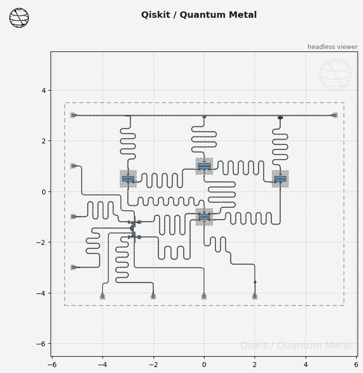
We can now run the simulation on the specified layout. All unconnected pins are left as shorts, as we are only concerned about simulating the resonant mode of the three components listed.
[39]:
eig_qb.sim.run(
    name="QMain_Q5_Bus05", components=["Q_Main", "Q5", "Bus_05"], open_terminations=[]
)
INFO 09:55AM [connect_project]: Connecting to Ansys Desktop API...
INFO 09:55AM [load_ansys_project]:      Opened Ansys App
INFO 09:55AM [load_ansys_project]:      Opened Ansys Desktop v2020.2.0
INFO 09:55AM [load_ansys_project]:      Opened Ansys Project
        Folder:    C:/Ansoft/
        Project:   Project23
INFO 09:55AM [connect_design]:  Opened active design
        Design:    Q_Main_q3d [Solution type: Q3D]
INFO 09:55AM [get_setup]:       Opened setup `Setup`  (<class 'pyEPR.ansys.AnsysQ3DSetup'>)
INFO 09:55AM [connect]:         Connected to project "Project23" and design "Q_Main_q3d" 😀

INFO 09:55AM [connect_design]:  Opened active design
        Design:    QMain_Q5_Bus05_hfss [Solution type: Eigenmode]
WARNING 09:55AM [connect_setup]:        No design setup detected.
WARNING 09:55AM [connect_setup]:        Creating eigenmode default setup.
INFO 09:55AM [get_setup]:       Opened setup `Setup`  (<class 'pyEPR.ansys.HfssEMSetup'>)
INFO 09:55AM [get_setup]:       Opened setup `3Modes`  (<class 'pyEPR.ansys.HfssEMSetup'>)
INFO 09:55AM [analyze]: Analyzing setup 3Modes
09:59AM 09s INFO [get_f_convergence]: Saved convergences to C:\workspace\qiskit-metal\docs\circuit-examples\full-design-flow-examples\hfss_eig_f_convergence.csv
Once the simulation is complete, we can check to see if the convergence was good.
[ ]:
eig_qb.sim.plot_convergences()
With the eigenmode simulation complete (and nicely converged) we can run some EPR analysis on the result.
At first we need to define the junctions in terms of name, inductance_variable, capacitance_variable, rectancle that was defined in the rendering to represent the junction port and line that was defined in the rendering to represent the direction of the current thorugh the junction.
[41]:
eig_qb.del_junction()
eig_qb.add_junction(
    "jj1", "Lj1", "Cj1", rect="JJ_rect_Lj_Q_Main_rect_jj", line="JJ_Lj_Q_Main_rect_jj_"
)
eig_qb.add_junction(
    "jj2", "Lj2", "Cj2", rect="JJ_rect_Lj_Q5_rect_jj", line="JJ_Lj_Q5_rect_jj_"
)
eig_qb.setup.sweep_variable = "Lj1"
eig_qb.setup
[41]:
{'junctions': {'jj1': {'Lj_variable': 'Lj1',
   'Cj_variable': 'Cj1',
   'rect': 'JJ_rect_Lj_Q_Main_rect_jj',
   'line': 'JJ_Lj_Q_Main_rect_jj_'},
  'jj2': {'Lj_variable': 'Lj2',
   'Cj_variable': 'Cj2',
   'rect': 'JJ_rect_Lj_Q5_rect_jj',
   'line': 'JJ_Lj_Q5_rect_jj_'}},
 'dissipatives': {'dielectrics_bulk': ['main']},
 'cos_trunc': 8,
 'fock_trunc': 7,
 'sweep_variable': 'Lj1'}
Note in the previous cell output that the dissipatives have alrady been defined by default.
Now we can start looking at the EPR values. First we look at the electric field and subtrate participation. Then extract the kerr matrix.
[42]:
eig_qb.run_epr()
# (pyEPR allows to switch modes: eprd.set_mode(1))
Design "QMain_Q5_Bus05_hfss" info:
        # eigenmodes    3
        # variations    1
Design "QMain_Q5_Bus05_hfss" info:
        # eigenmodes    3
        # variations    1

        energy_elec_all       = 5.30807060349227e-24
        energy_elec_substrate = 4.86434514599116e-24
        EPR of substrate = 91.6%

        energy_mag    = 2.32419129800195e-26
        energy_mag % of energy_elec_all  = 0.4%


Variation 0  [1/1]

  Mode 0 at 4.81 GHz   [1/3]
    Calculating ℰ_magnetic,ℰ_electric
       (ℰ_E-ℰ_H)/ℰ_E       ℰ_E       ℰ_H
               99.6%  2.654e-24 1.162e-26

    Calculating junction energy participation ration (EPR)
        method=`line_voltage`. First estimates:
        junction        EPR p_0j   sign s_0j    (p_capacitive)
                Energy fraction (Lj over Lj&Cj)= 97.68%
        jj1             3.29205e-06  (+)        7.83062e-08
                Energy fraction (Lj over Lj&Cj)= 97.33%
        jj2             0.994398  (+)        0.0272922
                (U_tot_cap-U_tot_ind)/mean=1.41%
Calculating Qdielectric_main for mode 0 (0/2)
p_dielectric_main_0 = 0.9164055095255939

  Mode 1 at 7.39 GHz   [2/3]
    Calculating ℰ_magnetic,ℰ_electric
       (ℰ_E-ℰ_H)/ℰ_E       ℰ_E       ℰ_H
                0.1%  3.353e-24  3.35e-24

    Calculating junction energy participation ration (EPR)
        method=`line_voltage`. First estimates:
        junction        EPR p_1j   sign s_1j    (p_capacitive)
                Energy fraction (Lj over Lj&Cj)= 94.69%
        jj1             0.000383918  (+)        2.15125e-05
                Energy fraction (Lj over Lj&Cj)= 93.93%
        jj2             0.000723443  (+)        4.6774e-05
                (U_tot_cap-U_tot_ind)/mean=0.00%
Calculating Qdielectric_main for mode 1 (1/2)
p_dielectric_main_1 = 0.9185431895828703

  Mode 2 at 14.79 GHz   [3/3]
    Calculating ℰ_magnetic,ℰ_electric
       (ℰ_E-ℰ_H)/ℰ_E       ℰ_E       ℰ_H
                0.0%  2.501e-24 2.501e-24

    Calculating junction energy participation ration (EPR)
        method=`line_voltage`. First estimates:
        junction        EPR p_2j   sign s_2j    (p_capacitive)
                Energy fraction (Lj over Lj&Cj)= 81.67%
        jj1             5.19757e-05  (+)        1.16685e-05
                Energy fraction (Lj over Lj&Cj)= 79.43%
        jj2             8.11545e-05  (+)        2.1022e-05
                (U_tot_cap-U_tot_ind)/mean=0.00%
Calculating Qdielectric_main for mode 2 (2/2)
p_dielectric_main_2 = 0.91725087597056
WARNING 09:59AM [__init__]: <p>Error: <class 'IndexError'></p>
ANALYSIS DONE. Data saved to:

C:\data-pyEPR\Project23\QMain_Q5_Bus05_hfss\2021-07-20 09-59-11.npz


         Differences in variations:


 . . . . . . . . . . . . . . . . . . . . . . . . . . . . . . . . . . . . . . . .
Variation 0

Starting the diagonalization
Finished the diagonalization
Pm_norm=
modes
0    1.028611
1    1.031457
2    1.123854
dtype: float64

Pm_norm idx =
     jj1    jj2
0  False   True
1  False  False
2  False  False
*** P (participation matrix, not normlz.)
        jj1       jj2
0  0.000003  0.967980
1  0.000384  0.000723
2  0.000052  0.000081

*** S (sign-bit matrix)
   s_jj1  s_jj2
0      1      1
1      1      1
2      1      1
*** P (participation matrix, normalized.)
   3.2e-06        1
   0.00038  0.00072
   5.2e-05  8.1e-05

*** Chi matrix O1 PT (MHz)
    Diag is anharmonicity, off diag is full cross-Kerr.
       264    0.588    0.132
     0.588 0.000408 0.000191
     0.132 0.000191 2.24e-05

*** Chi matrix ND (MHz)
       298      0.5    0.116
       0.5 0.000317 0.000173
     0.116 0.000173 2.28e-05

*** Frequencies O1 PT (MHz)
0     4550.033083
1     7388.261062
2    14788.982401
dtype: float64

*** Frequencies ND (MHz)
0     4533.470356
1     7388.272216
2    14788.988393
dtype: float64

*** Q_coupling
Empty DataFrame
Columns: []
Index: [0, 1, 2]
Mode frequencies (MHz)
Numerical diagonalization
| Lj1 | 13 |
|---|---|
| eigenmode | |
| 0 | 4550.03 |
| 1 | 7388.26 |
| 2 | 14788.98 |
Kerr Non-linear coefficient table (MHz)
Numerical diagonalization
| 0 | 1 | 2 | ||
|---|---|---|---|---|
| Lj1 | ||||
| 13 | 0 | 297.70 | 5.00e-01 | 1.16e-01 |
| 1 | 0.50 | 3.17e-04 | 1.73e-04 | |
| 2 | 0.12 | 1.73e-04 | 2.28e-05 |
From the analysis results we can determine the qubits anharmonicities and coupling strength. Once the analysis and tuning is complete, we can close the connection to Ansys.
[ ]:
eig_qb.sim.close()
Rendering to a GDS File
Once all of the tuning is complete, we will want to prepare a GDS file so we can create a mask and fabricate our chip. We first create a gds render instance.
[27]:
full_chip_gds = design.renderers.gds
The various options for the gds renderer can also be checked and changed as necessary. A key option is the gds file which holds the cells for your junction ebeam design. Make sure this is pointing at the correct file so they are placed in your final mask at the appropriate locations.
[28]:
full_chip_gds.options
[28]:
{'short_segments_to_not_fillet': 'True',
 'check_short_segments_by_scaling_fillet': '2.0',
 'gds_unit': 0.001,
 'ground_plane': 'True',
 'negative_mask': {'main': []},
 'fabricate': 'False',
 'corners': 'natural',
 'tolerance': '0.00001',
 'precision': '0.000000001',
 'width_LineString': '10um',
 'path_filename': '../resources/Fake_Junctions.GDS',
 'junction_pad_overlap': '5um',
 'max_points': '199',
 'cheese': {'datatype': '100',
  'shape': '0',
  'cheese_0_x': '25um',
  'cheese_0_y': '25um',
  'cheese_1_radius': '100um',
  'view_in_file': {'main': {1: True}},
  'delta_x': '100um',
  'delta_y': '100um',
  'edge_nocheese': '200um'},
 'no_cheese': {'datatype': '99',
  'buffer': '25um',
  'cap_style': '2',
  'join_style': '2',
  'view_in_file': {'main': {1: True}}},
 'bounding_box_scale_x': '1.2',
 'bounding_box_scale_y': '1.2'}
[29]:
full_chip_gds.options["path_filename"] = "../../tut/resources/Fake_Junctions.GDS"
full_chip_gds.options["no_cheese"]["buffer"] = "50um"
[30]:
full_chip_gds.export_to_gds("Full_Chip_01.gds")
11:09PM 01s INFO [import_junction_gds_file]: Rescaling imported junction library from unit=1e-06 to unit=0.001 (scale factor=0.001).
[30]:
1
(optional) With the design complete, we can close the GUI.
[ ]:
# gui.main_window.close()
For more information, review the Introduction to Quantum Computing and Quantum Hardware lectures below
|
Lecture Video | Lecture Notes | Lab |
|
Lecture Video | Lecture Notes | Lab |
|
Lecture Video | Lecture Notes | Lab |
|
Lecture Video | Lecture Notes | Lab |
|
Lecture Video | Lecture Notes | Lab |
|
Lecture Video | Lecture Notes | Lab |