Note

This page was generated from tut/2-From-components-to-chip/FlipChip-design-tutorial.ipynb.

Flip-Chip Devices in Quantum Metal

This notebook builds a qubit–resonator pair in a flip-chip stack and then analyzes it with the energy-participation-ratio (EPR) method.

The stack has two chips facing each other a few micrometers apart. Here the readout resonator sits on the bottom chip, called the control chip (C_chip), and the qubit on the top chip, the qubit chip (Q_chip); other layouts put both on one chip or split them differently.

# In Colab / Binder, uncomment to install Quantum Metal (lite, no Qt).
# Locally you should already have it via `pip install quantum-metal` or
# `pip install 'quantum-metal[gui]'` for the desktop GUI.
# !pip install -q quantum-metal

💡 Desktop GUI or inline. metal.gui(design) opens the desktop MetalGUI when Qt and a display are available and falls back to an inline viewer (Colab, Binder, a server) with the same API, so gui.rebuild() and gui.screenshot() work in both. See 1.1 Quick start and `docs/headless-usage.rst <https://qiskit-community.github.io/qiskit-metal/headless-usage.html>`__.

Section 1 (the layout) runs anywhere. Sections 2 and 3 add a material to Ansys and run an HFSS eigenmode simulation with EPR analysis; they need Ansys HFSS with pyEPR on Windows, and the cells that talk to Ansys are shown here without outputs.

🧭 Other simulation pathways. This notebook uses Ansys, which needs a license. Without one, the same kind of result can come from the open-source ElmerFEM path for capacitance (tutorial 4.19) or the pip-installable gmsh + scikit-fem solver for eigenmodes, couplings and capacitance (tutorials 4.43–4.45); AWS Palace is available through SQDMetal, with a native integration in progress. Simulation pathways summarizes what each solver computes, how to install it, and which tutorials use it.

1. Building a flip-chip design

DesignFlipChip works like DesignPlanar, except that it has two chips and each component says which one it is drawn on with its chip option. The two chips are called C_chip and Q_chip.

import qiskit_metal as metal
from qiskit_metal import Dict, designs
from qiskit_metal.qlibrary.qubits.transmon_cross import TransmonCross
from qiskit_metal.qlibrary.resonators.readoutres_fc import ReadoutResFC

design = designs.DesignFlipChip()
design.metadata["design_name"] = "FlipChip_Device"
# Allow re-running a cell to overwrite components with the same name
design.overwrite_enabled = True

gui = metal.gui(design)

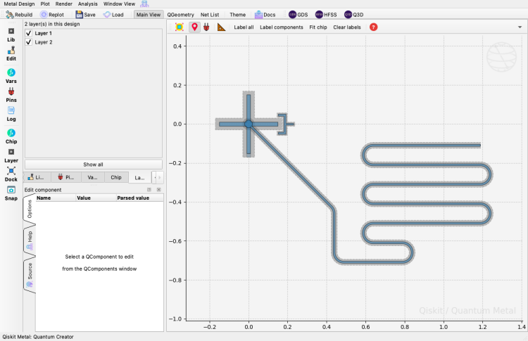
Next, we draw an Xmon on the Q-chip, and a readout resonator on the C-chip.

# delete existing components
design.delete_all_components()

# Draw an Xmon on the Q_chip: the `chip` option selects the chip.
options_cpads = Dict(
    connector_type="0",  # claw type
    claw_length="30um",
    ground_spacing="5um",
    claw_width="10um",
    claw_gap="6um",
)
options = Dict(
    chip="Q_chip",
    cross_width="20um",
    cross_length="150um",
    cross_gap="20um",
    connection_pads=Dict(claw_west=Dict(connector_location="180", **options_cpads)),
)

# position the center of the Xmon at (0,0)
q1_x = "0.0 mm"
q1_y = "0.0 mm"

# build the device, positioned at (q1_x, q1_y)
q1 = TransmonCross(design, "Q1", options=Dict(pos_x=q1_x, pos_y=q1_y, **options))

# rebuild in gui
gui.rebuild()
gui.autoscale()

# Draw a readout resonator on the C_chip (chip='C_chip').
# The resonator can have any shape; this one is a lambda/4 CPW resonator.
# The open-ended end of the resonator has a circular shape with a radius of readout_radius. Change this radius to change the qubit-resonator coupling strength.
# The cpw_width and cpw_gap are the size of the signal line and the ground gap of the cpw transmission line.
# The parameters readout_l1 ... l5, are the lengths of various parts of the cpw.
# arc_step is the length of a line that approximates an arc.
options = Dict(
    chip="C_chip",
    readout_radius="20 um",
    readout_cpw_width="10 um",
    readout_cpw_gap="10 um",
    readout_cpw_turnradius="50 um",
    readout_l1="600 um",
    readout_l2="200 um",
    readout_l3="300 um",
    readout_l4="150 um",
    readout_l5="550 um",
    arc_step="5 um",
)

# the resonator is set to have its origin at the center of the circular patch.
# So we set the qubit and the resonator to share the same coordinate (q1_x, q1_y)
r1 = ReadoutResFC(design, "R1", options=Dict(pos_x=q1_x, pos_y=q1_y, **options))

# rebuild in gui
gui.rebuild()
gui.autoscale()
gui.screenshot()

2. Preparation before rendering in Ansys

As described before, we have specified two chips in the FlipChipDesign class, i.e. C_chip and Q_chip. This information is stored in the chips variables.

design.chips

{'C_chip': {'material': 'silicon',
  'layer_start': '0',
  'layer_end': '2048',
  'size': {'center_x': '0.0mm',
   'center_y': '0.0mm',
   'center_z': '0.0mm',
   'size_x': '9mm',
   'size_y': '9mm',
   'size_z': '-280um',
   'sample_holder_top': '890um',
   'sample_holder_bottom': '1650um'}},
 'Q_chip': {'material': 'silicon',
  'layer_start': '0',
  'layer_end': '2048',
  'size': {'center_x': '0.0mm',
   'center_y': '0.0mm',
   'center_z': '20 um',
   'size_x': '9mm',
   'size_y': '9mm',
   'size_z': '280um',
   'sample_holder_top': '890um',
   'sample_holder_bottom': '1650um'}}}

It is important to note that in terms of component rendering in ANSYS, the components are drawn on an XY plane with its Z-coordinate being defined by ‘center_z’. For the design object we just created, C_chip components are drawn at z=0, and the Q_chip components are drawn at 20 um.

design.chips["C_chip"]["size"]["center_z"]

'0.0mm'

design.chips["Q_chip"]["size"]["center_z"]

'20 um'

Next, we set the Q_chip to be at a distance of, say 10 um, from the C_chip.

design.chips["Q_chip"]["size"]["center_z"] = "10 um"
design.chips["Q_chip"]["size"]["center_z"]

'10 um'

You may want a different substrate material. Rather than modifying an existing material, define a new one in the Ansys material library. If you don’t need this, skip to the next section.

For example, silicon with a dielectric constant of 11.45 instead of the default 11.9, called Si_11.45. First add it to the Ansys material library (by hand, or with the script below, which needs a running Ansys HFSS), then assign it to the chips in the design.

# new material properties
newMaterial_name = "Si_11.45"
newMaterial_permittivity = "11.45"
newMaterial_losstangent = "1e-7"

# Add the new material to the open Ansys project (needs Ansys HFSS).
from pyEPR import ansys, project_info

# get the handles to the ANSYS system
ans_prj = project_info.ProjectInfo()
oProject = ans_prj.project._project
defmanager = oProject.GetDefinitionManager()
# check if the material exists
if not defmanager.DoesMaterialExist(newMaterial_name):
    defmanager.AddMaterial(
        [
            "NAME:%s" % (newMaterial_name),
            "CoordinateSystemType:=",
            "Cartesian",
            "BulkOrSurfaceType:=",
            1,
            ["NAME:PhysicsTypes", "set:=", ["Electromagnetic"]],
            "permittivity:=",
            "%s" % (newMaterial_permittivity),
            "dielectric_loss_tangent:=",
            "%s" % (newMaterial_losstangent),
        ]
    )
# release the handle to ANSYS
ans_prj.project.release()
ans_prj.desktop.release()
ans_prj.app.release()
ansys.release()

# Specify the new material assignment for the chip
design.chips["C_chip"]["material"] = newMaterial_name
design.chips["Q_chip"]["material"] = newMaterial_name

3. Run EPR analysis

The EPR analysis follows tutorial 4.02 Eigenmode and EPR. First create an EPRanalysis object and update the HFSS simulation setup; this part runs without Ansys.

from qiskit_metal.analyses.quantization import EPRanalysis

eig_fc = EPRanalysis(design, "hfss")
eig_fc.sim.setup

{'name': 'Setup',
 'reuse_selected_design': True,
 'reuse_setup': True,
 'min_freq_ghz': 1,
 'n_modes': 1,
 'max_delta_f': 0.5,
 'max_passes': 10,
 'min_passes': 1,
 'min_converged': 1,
 'pct_refinement': 30,
 'basis_order': 1,
 'vars': {'Lj': '10 nH', 'Cj': '0 fF'}}

# update setup setting
eig_fc.sim.setup.max_passes = 20
eig_fc.sim.setup.vars.Lj = "10 nH"
# since we are analysing both the qubit and the resonator, we set the number of modes to be 2
eig_fc.sim.setup.n_modes = 2
# if there is not enough computational power, you can set a less stringent max_delta_f
eig_fc.sim.setup.max_delta_f = 1
eig_fc.sim.setup.min_freq_ghz = 1.5
# pass the name of the junction (for the EPR analysis purpose)
eig_fc.setup.junctions.jj.rect = "JJ_rect_Lj_Q1_rect_jj"
eig_fc.setup.junctions.jj.line = "JJ_Lj_Q1_rect_jj_"

eig_fc.sim.setup

{'name': 'Setup',
 'reuse_selected_design': True,
 'reuse_setup': True,
 'min_freq_ghz': 1.5,
 'n_modes': 2,
 'max_delta_f': 1,
 'max_passes': 20,
 'min_passes': 1,
 'min_converged': 1,
 'pct_refinement': 30,
 'basis_order': 1,
 'vars': {'Lj': '10 nH', 'Cj': '0 fF'}}

Then run the HFSS simulation and the EPR analysis. These cells need Ansys HFSS and are shown without outputs.

eig_fc.sim.run(
    name="qubitres", components=["Q1", "R1"], open_terminations=[], box_plus_buffer=True
)

eig_fc.setup.dissipatives.dielectrics_bulk = ["Q_chip", "C_chip"]
eig_fc.run_epr()

eig_fc.sim.close()

For more information, review the Introduction to Quantum Computing and Quantum Hardware lectures below

Superconducting Qubits I: Quantizing a Harmonic Oscillator, Josephson Junctions Part 1	Lecture Video	Lecture Notes	Lab
Superconducting Qubits I: Quantizing a Harmonic Oscillator, Josephson Junctions Part 2	Lecture Video	Lecture Notes	Lab
Superconducting Qubits I: Quantizing a Harmonic Oscillator, Josephson Junctions Part 3	Lecture Video	Lecture Notes	Lab
Superconducting Qubits II: Circuit Quantum Electrodynamics, Readout and Calibration Methods Part 1	Lecture Video	Lecture Notes	Lab
Superconducting Qubits II: Circuit Quantum Electrodynamics, Readout and Calibration Methods Part 2	Lecture Video	Lecture Notes	Lab
Superconducting Qubits II: Circuit Quantum Electrodynamics, Readout and Calibration Methods Part 3	Lecture Video	Lecture Notes	Lab