Note
This page was generated from tut/4-Analysis/pyaedt-multiplanar/DrivenModal-pyaedt-multiplanar.ipynb.
HFSS Driven Modal Simulation of a MultiPlanar Design with pyaedt
A MultiPlanar design reads its layers from a layer-stack file: for each layer, its z position, thickness, material and whether it is filled. The pyaedt renderers use that stack to build the 3D model in Ansys.
Note: this may work only with the full (paid) version of Ansys, not the student version. This issue is fixable and requires more testing. Please run the notebook and test it out on student license, if you’re interested to make a contribution!


💡 Desktop GUI or inline.
metal.gui(design)opens the desktopMetalGUIwhen Qt and a display are available and falls back to an inline viewer (Colab, Binder, a server) with the same API, sogui.rebuild()andgui.screenshot()work in both. See 1.1 Quick start and`docs/headless-usage.rst<https://qiskit-community.github.io/qiskit-metal/headless-usage.html>`__.Everything up to and including the layout runs anywhere. The rest drives Ansys through pyaedt (HFSS driven modal: setup, frequency sweep, S-parameters); those cells need Ansys Electronics Desktop and are shown here without outputs.
🧭 Other simulation pathways. This notebook uses Ansys, which needs a license. Without one, the same kind of result can come from the open-source ElmerFEM path for capacitance (tutorial 4.19) or the pip-installable gmsh + scikit-fem solver for eigenmodes, couplings and capacitance (tutorials 4.43–4.45); AWS Palace is available through SQDMetal, with a native integration in progress. Simulation pathways summarizes what each solver computes, how to install it, and which tutorials use it.
[2]:
import qiskit_metal as metal
from qiskit_metal import Dict
from qiskit_metal.designs.design_multiplanar import MultiPlanar
from qiskit_metal.renderers.renderer_ansys_pyaedt.hfss_renderer_drivenmodal_aedt import (
    QHFSSDrivenmodalPyaedt,
)
Layer stack
The layer stack is a CSV file with one row per layer and datatype.
[3]:
# The example stack ships with the tutorials, in docs/tut/resources/.
ls_file_path = "../../resources/layer_stack_data_example_1.csv"

multiplanar_design = MultiPlanar(
    metadata={}, overwrite_enabled=True, layer_stack_filename=ls_file_path
)
Multi-Planar design has default of chip named main. If there is more than one, add information to multiplanar design.
[4]:
multiplanar_design._chips.main.size.size_x = "7mm"
multiplanar_design._chips.main.size.size_y = "7mm"
multiplanar_design._chips["qubit_chip"] = Dict()
multiplanar_design._chips.qubit_chip.size = Dict(
    center_x="0.0mm",
    center_y="0.0mm",
    size_x="7mm",
    size_y="7mm",
)


# Override the default values size for chip=='main'.
multiplanar_design.chips.main.size["size_x"] = "2mm"
multiplanar_design.chips.main.size["size_y"] = "2mm"
[5]:
multiplanar_design.chips
[5]:
{'main': {'size': {'center_x': '0.0mm',
   'center_y': '0.0mm',
   'size_x': '2mm',
   'size_y': '2mm'}},
 'qubit_chip': {'size': {'center_x': '0.0mm',
   'center_y': '0.0mm',
   'size_x': '7mm',
   'size_y': '7mm'}}}
[6]:
# Remember, the layers may not always be unique, since there can be multiple datatypes.
ls_unique = multiplanar_design.ls.is_layer_data_unique()
Open the GUI on the MultiPlanar design
[7]:
gui = metal.gui(multiplanar_design)
Add all components to design.
Note the layer number and chip names are used when adding components to design.
[8]:
from qiskit_metal.qlibrary.qubits.transmon_pocket import TransmonPocket
from qiskit_metal.qlibrary.terminations.open_to_ground import OpenToGround
from qiskit_metal.qlibrary.tlines.meandered import RouteMeander
from qiskit_metal.qlibrary.qubits.transmon_concentric import TransmonConcentric

from qiskit_metal.qlibrary.couplers.coupled_line_tee import CoupledLineTee
from qiskit_metal.qlibrary.tlines.straight_path import RouteStraight

# As precaution, remove any components already previously to design.
multiplanar_design.delete_all_components()

qubit_cpw_otg_layer = 2
qubit_chip_name = "qubit_chip"


##############################################################################


options = dict(
    # Some options we want to modify from the defaults
    pad_width="425 um",
    pocket_height="650um",
    layer=qubit_cpw_otg_layer,
    chip=qubit_chip_name,
    # Adding 4 connectors (see below for defaults)
    connection_pads=dict(
        a=dict(loc_W=+1, loc_H=+1),
        b=dict(loc_W=-1, loc_H=+1, pad_height="30um"),
        c=dict(loc_W=+1, loc_H=-1, pad_width="200um"),
        d=dict(loc_W=-1, loc_H=-1, pad_height="50um"),
    ),
)

## Create 2 transmons

q1 = TransmonPocket(
    multiplanar_design,
    "Q1",
    options=dict(pos_x="+1.4mm", pos_y="0mm", orientation="90", **options),
)
q2 = TransmonPocket(
    multiplanar_design,
    "Q2",
    options=dict(pos_x="-0.6mm", pos_y="0mm", orientation="90", **options),
)

##############################################################################

TQ1 = CoupledLineTee(
    multiplanar_design,
    "TQ1",
    options=dict(
        pos_x="1mm",
        pos_y="3mm",
        layer=qubit_cpw_otg_layer,
        chip=qubit_chip_name,
        coupling_length="200um",
    ),
)
TQ2 = CoupledLineTee(
    multiplanar_design,
    "TQ2",
    options=dict(
        pos_x="-1mm",
        pos_y="3mm",
        layer=qubit_cpw_otg_layer,
        chip=qubit_chip_name,
        coupling_length="200um",
    ),
)

##############################################################################

ops = dict(fillet="90um")
multiplanar_design.overwrite_enabled = True

options1 = Dict(
    total_length="8mm",
    hfss_wire_bonds=True,
    layer=qubit_cpw_otg_layer,
    chip=qubit_chip_name,
    pin_inputs=Dict(
        start_pin=Dict(component="TQ1", pin="second_end"),
        end_pin=Dict(component="Q1", pin="a"),
    ),
    lead=Dict(start_straight="0.1mm"),
    **ops,
)

options2 = Dict(
    total_length="9mm",
    hfss_wire_bonds=True,
    layer=qubit_cpw_otg_layer,
    chip=qubit_chip_name,
    pin_inputs=Dict(
        start_pin=Dict(component="TQ2", pin="second_end"),
        end_pin=Dict(component="Q2", pin="a"),
    ),
    lead=Dict(start_straight="0.1mm"),
    **ops,
)

meanderQ1 = RouteMeander(multiplanar_design, "meanderQ1", options=options1)
meanderQ2 = RouteMeander(multiplanar_design, "meanderQ2", options=options2)

##############################################################################

otg1 = OpenToGround(
    multiplanar_design,
    "otg1",
    options=dict(
        pos_x="3mm", layer=qubit_cpw_otg_layer, chip=qubit_chip_name, pos_y="3mm"
    ),
)
otg2 = OpenToGround(
    multiplanar_design,
    "otg2",
    options=dict(
        pos_x="-3mm",
        pos_y="3mm",
        layer=qubit_cpw_otg_layer,
        chip=qubit_chip_name,
        orientation="180",
    ),
)

##############################################################################

ops_oR = Dict(
    hfss_wire_bonds=True,
    layer=qubit_cpw_otg_layer,
    chip=qubit_chip_name,
    pin_inputs=Dict(
        start_pin=Dict(component="TQ1", pin="prime_end"),
        end_pin=Dict(component="otg1", pin="open"),
    ),
)
ops_mid = Dict(
    hfss_wire_bonds=True,
    layer=qubit_cpw_otg_layer,
    chip=qubit_chip_name,
    pin_inputs=Dict(
        start_pin=Dict(component="TQ1", pin="prime_start"),
        end_pin=Dict(component="TQ2", pin="prime_end"),
    ),
)
ops_oL = Dict(
    hfss_wire_bonds=True,
    layer=qubit_cpw_otg_layer,
    chip=qubit_chip_name,
    pin_inputs=Dict(
        start_pin=Dict(component="TQ2", pin="prime_start"),
        end_pin=Dict(component="otg2", pin="open"),
    ),
)

cpw_openRight = RouteStraight(multiplanar_design, "cpw_openRight", options=ops_oR)
cpw_middle = RouteStraight(multiplanar_design, "cpw_middle", options=ops_mid)
cpw_openLeft = RouteStraight(multiplanar_design, "cpw_openLeft", options=ops_oL)

##############################################################################

# Place the concentric transmon within design.
concentric_options = dict(
    # chip='main',
    pos_x="400um",
    pos_y="900um",
    # layer='1',  # default is 1, this is just for example.
    pocket_w="1500um",  # transmon pocket width
    pocket_h="900um",  # transmon pocket height
)

# Create a new Concentric Transmon object with name 'Q1'
qc1 = TransmonConcentric(multiplanar_design, "cc_qubit", options=concentric_options)

gui.rebuild()
gui.autoscale()
gui.screenshot()
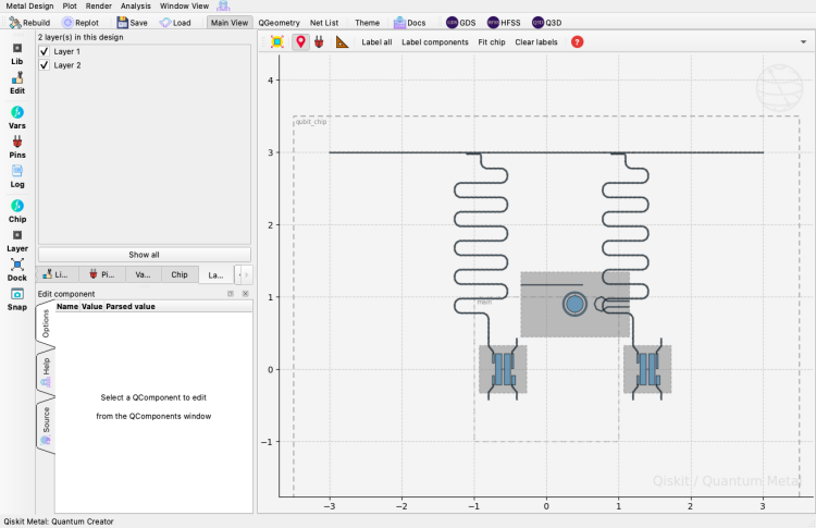
Start the HFSS Driven Modal renderer for Ansys by passing arguments to QHFSSDrivenmodalPyaedt.
The default will use default names for Ansys ProjectName and Ansys DesignName.
[9]:
# Ansys will not start here since default for initiate is False.

# Example with defaults.
# hfss_dm_default = QHFSSDrivenmodalPyaedt(multiplanar_design)

hfss_dm = QHFSSDrivenmodalPyaedt(
    multiplanar_design, "hfss_dm_project_1", "hfss_dm_design_1"
)

# # Ansys will start here.
# hfss_dm_2 = QHFSSDrivenmodalPyaedt(multiplanar_design,
#                                    'hfss_dm_project_2',
#                                    'hfss_dm_design_2',
#                                    initiate=True)
Vacuum Box size given to renderer.
[10]:
# Sample Holder options will determine the z values of vacuum box.
hfss_dm.options["sample_holder_top"] = "1.0mm"
hfss_dm.options["sample_holder_bottom"] = "-1.0mm"

# Note, the xy size of vacuum box is determined by box_plus_buffer.
# If False, the chip size will be used.
# If True, a buffer will be added to the box which contains the rendered components.
Examine arguments to pass for Ansys-setup for driven modal.
[11]:
"""Create a solution setup in Ansys HFSS Driven-Modal solution type. If user does not provide
    arguments, they will be obtained from QHFSSDrivenmodalPyaedt.default_setup dict.

    Args:
        name (str, optional): _description_. Defaults to None.
        SolveType (str, optional): Solution frequency type. Accepted values are in self.__supported_SolveType__.
                                Defaults to self.default_setup.
        Frequency (float, optional):  Minimum frequency in GHz. Defaults to self.default_setup.
        MaxDeltaE (float, optional):  This is correlated to MaxDeltaS. The definition
                                of MaxDeltaS is, absolute value of maximum difference in
                                scattering parameter S. Defaults to self.default_setup.
        MaximumPasses (int, optional):  Maximum number of passes. Defaults to self.default_setup.
        MinimumPasses (int, optional): Minimum number of passes.Defaults to self.default_setup.
        MinimumConvergedPasses (int, optional): Minimum number of converged passes. Defaults to self.default_setup.
        PercentRefinement (int, optional): Percent refinement. Defaults to self.default_setup.
        BasisOrder (int, optional): Basis order. Defaults to self.default_setup.
        MultipleAdaptiveFreqsSetup (dict, optional): Frequencies and their associated MaxDeltaS.
                                Defaults to self.default_setup.
        BroadbandLowFreq (float, optional): Minimum frequency for Broadband SolveType in GHz.
                                Defaults to self.default_setup.
        BroadbandHighFreq (float, optional): Maximum frequency for Broadband SolveType in GHz.
                                Defaults to self.default_setup.

    Returns:
        new_setup (pyaedt.modules.SolveSetup.SetupHFSS): pyAEDT simulation setup object.
"""

hfss_dm.default_setup
[11]:
{'name': 'QHFSSDrivenmodalPyaedt_setup',
 'SolveType': 'Single',
 'Frequency': '5.0',
 'MaxDeltaE': '0.01',
 'MaximumPasses': '10',
 'MinimumPasses': '1',
 'MinimumConvergedPasses': '1',
 'PercentRefinement': '30',
 'BasisOrder': '1',
 'MultipleAdaptiveFreqsSetup': {'1GHz': [0.02],
  '2GHz': [0.02],
  '5GHz': [0.02]},
 'BroadbandLowFreq': '2',
 'BroadbandHighFreq': '8'}
Add solution setup to Ansys Driven Modal.
[ ]:
# Ansys should add project and design for hfss_dm.
hfss_dm.add_hfss_dm_setup()

# Reduce MaxPass when running notebook as an example.
hfss_dm.add_hfss_dm_setup(name="fun_dm_1", MaximumPasses=3)


#### We have access to other solution frequency types as well
#### Normally it defaults to `SolveType=Single` (single frequency).

## 1. Multiple Frequencies
# multiple_freqs = OrderedDict([('4GHz', [0.01]),
#                               ('6GHz', [0.001]),
#                               ('11GHz', [0.0001])])
# hfss_dm.add_hfss_dm_setup(
#     name=None,
#     SolveType='MultiFrequency'
#     MultipleAdaptiveFreqsSetup=multiple_freqs)

## 2. Broadband
# hfss_dm.add_hfss_dm_setup(
#     name=None,
#     SolveType='Broadband',
#     BroadbandLowFreq="4",  # GHz
#     BroadbandHighFreq="11"  # GHz
# )
Since user can edit the GUI, it is “better” to clean the user’s project and design denoted when starting the renderer.
[ ]:
hfss_dm.clean_user_design()
Render the multi-planar design using the similar convention as planar-design to identify ports.
[ ]:
hfss_dm.render_design(
    selection=["TQ1", "TQ2", "cpw_openRight", "cpw_openLeft", "cpw_middle", "Q1", "Q2"],
    open_pins=[],
    port_list=[("cpw_openRight", "end", 50), ("cpw_openLeft", "end", 50)],
    jj_to_port=[("Q2", "rect_jj", 51)],
    ignored_jjs=[("Q1", "rect_jj")],
    box_plus_buffer=True,
)
Examine arguments to pass for Ansys-sweep for driven modal.
Add a frequency sweep to a driven modal setup.

Args:
    setup_name (str, optional): Name of driven modal simulation setup.
                            Defaults to "QHFSSDrivenmodalPyaedt_setup".
    unit(str, optional): The units of start and stop.
    start_ghz (float, optional): Starting frequency of sweep in GHz.
                            Defaults to 2.0.
    stop_ghz (float, optional): Ending frequency of sweep in GHz.
                            Defaults to 8.0.
    count (int, optional): Total number of frequencies.
                            Defaults to 101.
    step_ghz (float, optional): Difference between adjacent
                            frequencies. Defaults to None.
    name (str, optional): Name of sweep. Defaults to "QHFSSDrivenmodalPyaedt_sweep".
    type (str, optional): Type of sweep.  Options are "Fast", "Interpolating",
                        and "Discrete". Defaults to "Fast".
    save_fields (bool, optional): Whether or not to save fields.
                        Defaults to False.
    interpolation_tol (float, optional): Error tolerance threshold
                                for the interpolation type sweep. Defaults to 0.5.
    interpolation_max_solutions (int, optional): Maximum number of solutions
                                evaluted for the interpolation process.
                                Defaults to 250.
[ ]:
# Add sweep for specific setup and give new name for sweep.

hfss_dm.add_sweep(
    setup_name="fun_dm_1",
    name="fun_dm_1_sweep",
    start_ghz=4.0,
    stop_ghz=8.0,
    count=2001,
    type="Interpolating",
    interpolation_tol=0.1,
    interpolation_max_solutions=500,
)
Select the name to analyze. Presently, we have two to choose from.
They are default==’QHFSSDrivenmodalPyaedt_setup’ and ‘fun_dm_1’.
[ ]:
# This has some error checking before using pyaedt's analyze_setup.
result_bool = hfss_dm.analyze_setup(setup_name="fun_dm_1", sweep_name="fun_dm_1_sweep")
Get the solution data!
Can get scatter data, impedance, and admittance in format of mag/phase or real/imag.
Get the solution data based on expressions.  Return output based on output_type.

Args:
   sweep_name (str): Name of sweep entry within setup.
   expressions (str, optional): This expression is either passed to get_solution_data
                               OR either S, Y or Z with port information will be
                               gathered by renderer. The renderer will get the
                               port names used with render_design() to create expressions.
                               So, the user MUST execute render_design() prior to
                               getting solution data.

                               Defaults to 'S'. S for scattering, Y for admittance, Z for
                               impedance.
   output_type (int, optional): 1 to return mag/phase,
                               2 to return real/imag,
                               3 to return mag/phase and real/imag.
                               Defaults to 1.

Returns:
   dict: Key is either mag, phase, real or imag based on output_type.
       The value is data from get_solution_data.
[ ]:
result_dict_default = hfss_dm.get_ansys_solution_data(sweep_name="fun_dm_1_sweep")

# To make more viewable, print some lines.
print()
print()
result_dict_default.keys()
[ ]:
result_dict_s = hfss_dm.get_ansys_solution_data(
    sweep_name="fun_dm_1_sweep", expressions="S", output_type=3
)
# To make more viewable, print some lines.
print()
print()
result_dict_s.keys()
Remove the hash mark to retrieve the type of data you want to retrieve from Scatter Solution Data.
[12]:
# Remove comment to view all frequencies.
# result_dict_s

# Remove comment to view pandas dataframe for magnitude for all frequencies for scatter solution data.
# result_dict_s['mag']

# Remove comment to view pandas dataframe for real data for all frequencies for scatter solution data.
# result_dict_s['real']
[ ]:
# Example of getting impedance data.
result_dict_z = hfss_dm.get_ansys_solution_data(
    sweep_name="fun_dm_1_sweep", expressions="Z", output_type=3
)
result_dict_s["mag"]
[ ]:
# Will disconnect Metal from Ansys, and leave Ansys open.
# If the python script closes, the OS will most likely close Ansys.
# hfss_dm.close()


# Will close Ansys.
# hfss_dm.force_exit_ansys()
For more information, review the Introduction to Quantum Computing and Quantum Hardware lectures below
|
Lecture Video | Lecture Notes | Lab |
|
Lecture Video | Lecture Notes | Lab |
|
Lecture Video | Lecture Notes | Lab |
|
Lecture Video | Lecture Notes | Lab |
|
Lecture Video | Lecture Notes | Lab |
|
Lecture Video | Lecture Notes | Lab |