Note
This page was generated from tut/1-Overview/1.4-Headless-quick-view-(no-Qt-GUI).ipynb.
1.4 Headless Quick View — using Quantum Metal without the Qt GUI
This notebook shows how to design and view components in Quantum Metal without launching the Qt desktop GUI. The full API works headlessly in a plain Python interpreter or in cloud notebook environments like Jupyter, Colab, and Binder where Qt isn’t available or wanted.
What you’ll learn
How to build a design programmatically — same API as the GUI workflow
How to use
qm.view(design)to render a design to a matplotlib figure inlineHow to customise the view: filter components, hide layers, render into existing axes
How to save the rendered design to a file
When to use this workflow
You’re running on a server / cloud notebook (Colab, Binder, JupyterHub) where PySide6 isn’t installed.
You’re scripting a parameter sweep and just want to verify the geometry looks right.
You’re embedding Quantum Metal in a larger pipeline (CI, automated optimization, papers/figures).
If you want the interactive editor with click-to-select components, dockable panels, and live option editing, use qm.MetalGUI(design) instead. That requires a local installation with PySide6.
Setup
We force matplotlib’s Agg backend before any plot calls so the notebook works on headless runners. In a normal Jupyter session you can skip this — Jupyter picks an inline-friendly backend automatically.
[1]:
import matplotlib
from matplotlib import pyplot as plt

# matplotlib.use("Agg")  # only needed when not in Jupyter

import qiskit_metal as qm
from qiskit_metal import Dict
from qiskit_metal.designs import DesignPlanar
from qiskit_metal.qlibrary.qubits.transmon_pocket import TransmonPocket
from qiskit_metal.qlibrary.terminations.open_to_ground import OpenToGround
10:00PM 27s WARNING [_maybe_warn_lite_flip]: [FutureWarning] quantum-metal v0.7.0 will move PySide6, qdarkstyle, pyaedt, pyEPR-quantum, and gmsh out of base dependencies into opt-in extras. To preserve the current v0.6.x install behaviour, run `pip install 'quantum-metal[full]'` before upgrading. See ROADMAP.md and docs/migration-to-v0.7.0.rst for details. Set QISKIT_METAL_SUPPRESS_LITE_FLIP_WARNING=1 to silence.
Build a small design programmatically
Same API as the GUI workflow — no Qt window is created.
[2]:
design = DesignPlanar()

# A transmon qubit with one coupling pad
TransmonPocket(
    design,
    "Q1",
    options=Dict(
        pos_x="0mm",
        pos_y="0mm",
        connection_pads=Dict(
            a=Dict(loc_W="+1", loc_H="+1"),
        ),
    ),
)

# A ground termination next to it
OpenToGround(
    design,
    "G1",
    options=Dict(pos_x="1mm", pos_y="0mm"),
)

print("Components in design:", list(design.components.keys()))
Components in design: ['Q1', 'G1']
View the design
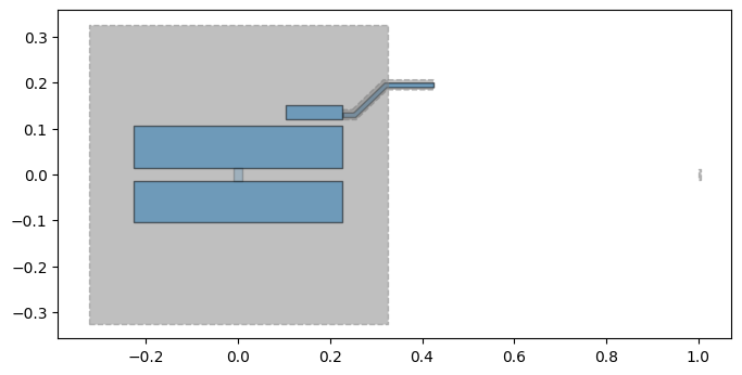
qm.view(design) returns a matplotlib.figure.Figure. In Jupyter it will display inline; you can also save it or further customise it like any other matplotlib figure.
[3]:
fig = qm.view(design)  # shows automatically in jupyter
fig  # You can also use "display(fig)"
[3]:
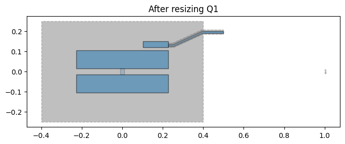
Iterating on the design
Changing a component’s options is the same workflow as in the GUI — but you get a new Figure instead of an updated Qt canvas. Component objects are accessible by name via design.components.
[4]:
# Change Q1's pocket dimensions and re-render — no Qt window
design.components["Q1"].options.pocket_width = "800um"
design.components["Q1"].options.pocket_height = "500um"
design.rebuild()

fig = qm.view(design, title="After resizing Q1")
fig
[4]:
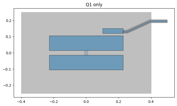
Customising the view
Filter to specific components
[5]:
fig = qm.view(design, components=["Q1"], title="Q1 only")
fig
[5]:
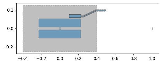
Custom figure size
[6]:
fig = qm.view(design, figsize=(6, 4))
fig
[6]:
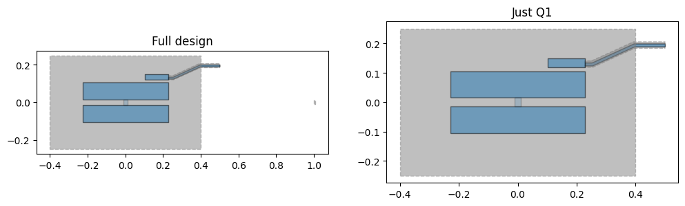
Side-by-side in a multi-panel figure
[7]:
import matplotlib.pyplot as plt

fig, axes = plt.subplots(1, 2, figsize=(12, 5))
qm.view(design, ax=axes[0], title="Full design")
qm.view(design, ax=axes[1], components=["Q1"], title="Just Q1")
fig
[7]:
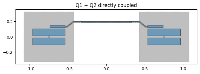
A coupled two-qubit design
The components= argument to qm.view lets you highlight any subset of the design — useful for inspecting individual qubits or the coupler in isolation. Here we build two TransmonPocket qubits connected by a RouteStraight bus coupler and then view them together and separately.
[8]:
from qiskit_metal.qlibrary.tlines.straight_path import RouteStraight

design2 = DesignPlanar()
design2.chips.main.size["size_x"] = "3mm"
design2.chips.main.size["size_y"] = "2mm"

TransmonPocket(
    design2,
    "Q1",
    options=Dict(
        pos_x="-0.75mm",
        pos_y="0mm",
        pad_width="425um",
        pocket_height="650um",
        connection_pads=Dict(
            readout=Dict(loc_W=+1, loc_H=+1, pad_width="200um"),
        ),
    ),
)

TransmonPocket(
    design2,
    "Q2",
    options=Dict(
        pos_x="0.75mm",
        pos_y="0mm",
        pad_width="425um",
        pocket_height="650um",
        connection_pads=Dict(
            readout=Dict(loc_W=-1, loc_H=+1, pad_width="200um"),
        ),
    ),
)

RouteStraight(
    design2,
    "coupler",
    Dict(
        pin_inputs=Dict(
            start_pin=Dict(component="Q1", pin="readout"),
            end_pin=Dict(component="Q2", pin="readout"),
        ),
    ),
)

print("Components:", list(design2.components.keys()))
Components: ['Q1', 'Q2', 'coupler']
[9]:
fig = qm.view(design2, title="Q1 + Q2 directly coupled")
fig
[9]:
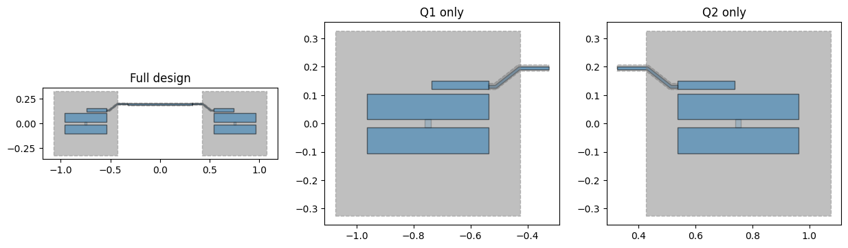
Highlight individual components
Pass components=[...] with any subset of component names. Everything else is hidden, so you can focus on one qubit, one coupler, or any combination.
[10]:
fig, axes = plt.subplots(1, 3, figsize=(15, 5))
qm.view(design2, ax=axes[0], title="Full design")
qm.view(design2, ax=axes[1], components=["Q1"], title="Q1 only")
qm.view(design2, ax=axes[2], components=["Q2"], title="Q2 only")
fig
[10]:
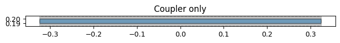
[11]:
# The coupler on its own — useful for checking routing geometry
fig = qm.view(design2, components=["coupler"], title="Coupler only")
fig
[11]:
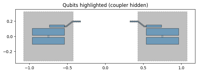
Highlight a subset — headless equivalent of gui.highlight_components()
In the Qt GUI you’d call gui.highlight_components(["Q1", "Q2"]) to focus on specific components. The headless equivalent is the same components= argument — pass any combination of component names and everything else is hidden.
[12]:
# Show both qubits together, hide the coupler
fig = qm.view(
    design2, components=["Q1", "Q2"], title="Qubits highlighted (coupler hidden)"
)
fig
[12]:
Interactive pan & zoom in JupyterLab
qm.view() returns a standard matplotlib Figure that works with any backend. Switch to the widget backend (powered by ipympl) for interactive pan, zoom, and mouse navigation directly inside JupyterLab.
Install ``ipympl`` if you do not have it:
pip install "quantum-metal[jupyter]"   # full dev install — already includes ipympl
pip install ipympl                      # standalone
Two rules for switching backends
Switch before you create any figures.
%matplotlib widgetregisters a new canvas type; figures already open stay on the old backend and won’t become interactive. Re-run the plot cells after switching.Qt and ipympl cannot share a kernel. If Qt has been initialised in this kernel session (e.g. you imported
MetalGUIearlier, even in a different notebook), the widget backend will silently accept the switch but figures will still render statically. In that case restart the kernel and run%matplotlib widgetas the very first cell.
This notebook never imports
MetalGUI, so the widget backend works here without a kernel restart. Notebooks that do useMetalGUI(e.g. 1.2, 1.3) cannot switch towidgetmid-session — use this notebook for interactive exploration instead.
(You may have to restart your kernel and run these cells first here)
[13]:
# Run this cell FIRST — before any qm.view() or plt calls.
# Re-run the plot cells below after switching to see the interactive canvas.
try:
    import ipympl  # noqa: F401

    get_ipython().run_line_magic("matplotlib", "widget")
    import matplotlib

    print(f"Backend switched to: {matplotlib.get_backend()}")
    print("Re-run the plot cells below to get interactive figures.")
except ImportError:
    get_ipython().run_line_magic("matplotlib", "inline")
    print("ipympl not installed — static inline figures only.")
    print('Install: pip install "quantum-metal[jupyter]"')
except Exception as e:
    get_ipython().run_line_magic("matplotlib", "inline")
    print(f"Could not switch to widget backend ({e}).")
    print("If Qt is active in this kernel, restart and run this cell first.")
Backend switched to: widget
Re-run the plot cells below to get interactive figures.
[14]:
# Now qm.view() returns an interactive figure: scroll to zoom, drag to pan
fig = qm.view(design2, title="Interactive view — use toolbar to zoom and pan")
# fig.show() - not needed
Interacting with the figure
The toolbar on the left edge of the canvas gives you full mouse control:
Button
Action
⌂ Home
Reset to the original view
← Back
Step back through previous views
→ Forward
Step forward through views
✥ Pan
Click and drag to pan around the design
□ Zoom
Draw a rectangle to zoom into that region
💾 Save
Download the current view as a PNG
You can also scroll (mouse wheel / trackpad pinch) to zoom in and out directly on the canvas.
Note: The interactive toolbar requires
ipympl(pip install "quantum-metal[jupyter]"). If you only see a static image, run%matplotlib widgetbefore any plotting cells, then re-run this cell.
[15]:
# Switch back to static inline rendering when you're done exploring
%matplotlib inline
Batch export: render multiple designs to PNG
Headless rendering shines when you want to automate exports — for example, generating figures for a paper or sweeping a parameter.
[ ]:
import os
import qiskit_metal as qm

%matplotlib inline

output_dir = "batch_output"
os.makedirs(output_dir, exist_ok=True)

# Vary Q1's pad_width across three values and save each view
for pad_w in ["300 um", "425 um", "550 um"]:
    design2.components["Q1"].options.pad_width = pad_w
    design2.rebuild()
    fig = qm.view(design2, title=f"pad_width = {pad_w}")
    safe_name = pad_w.replace(" ", "").replace("/", "_")
    fig.savefig(
        f"{output_dir}/design_pad_{safe_name}.png", dpi=150, bbox_inches="tight"
    )
    print(f"Saved design_pad_{safe_name}.png")

# Restore original
design2.components["Q1"].options.pad_width = "425 um"
design2.rebuild()
print("Done — check the batch_output/ folder")
Tip: Wrap this pattern in a function and loop over any option — qubit positions, CPW lengths, pad gaps. The PNG filenames become your experiment log.
Save to a file
Any matplotlib.figure.Figure method works — savefig to PNG/PDF/SVG, embed in a paper, etc.
[18]:
fig = qm.view(design)
fig.savefig("my_design.png", dpi=150, bbox_inches="tight")
print("Saved my_design.png")
Saved my_design.png
What about HFSS / Q3D / GDS?
All non-Qt renderers work headlessly too:
GDS export —
QGDSRenderer(design).export_to_gds("out.gds")works without Qt.HFSS / Q3D — the renderer doesn’t require Qt, but it does require Ansys AEDT installed on the machine running the script. On a cloud notebook without Ansys, you can still build the design and export GDS / visualise with
qm.view; you just can’t run the live solve.Analyses — every module in
qiskit_metal.analysesis pure Python (numpy / scipy / qutip) and works headlessly.
Next steps
See
docs/headless-usage.rstfor the full reference.See the 1.2 Quick start notebook for a tour of the GUI-driven workflow.
For interactive pan/zoom in Jupyter without Qt, install
ipympland run%matplotlib widgetat the top of your notebook.
What’s next
Browse 1.1 Bird’s eye view and 1.2 Quick start — they use
MetalGUIfor visualisation but every concept transfers; just replacegui.rebuild()withqm.view(design). The GUI-screenshots in those tutorials give you a sense of what the desktop experience looks like.See the 2 From components to chip folder for multi-qubit designs and CPW routing. The same
qm.view(design)call works for any of them — passfigsize=(12, 12)for chip-scale views.For programmatic GDS export (no Qt or Ansys required), use the
QGDSRenderer:from qiskit_metal.renderers.renderer_gds.gds_renderer import QGDSRenderer gds = QGDSRenderer(design) gds.export_to_gds("my_chip.gds")
Read the full reference in
`docs/headless-usage.rst<../../docs/headless-usage.rst>`__ for all ofqm.view’s options, the[gui]/[ansys]/[fem]install extras, and the roadmap for a future richer interactive viewer.
For more information, review the Introduction to Quantum Computing and Quantum Hardware lectures below
|
Lecture Video | Lecture Notes | Lab |
|
Lecture Video | Lecture Notes | Lab |
|
Lecture Video | Lecture Notes | Lab |
|
Lecture Video | Lecture Notes | Lab |
|
Lecture Video | Lecture Notes | Lab |
|
Lecture Video | Lecture Notes | Lab |