Optimize dual frame

This document shows you how to optimize the post-processing of the POVM samples to improve expectation value estimations.

%load_ext autoreload
%autoreload 2

Getting the POVM samples

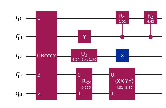
Define quantum circuit

from qiskit.circuit.random import random_circuit

qc = random_circuit(5, 3, measure=False, seed=875)
qc.draw("mpl", style="iqp")

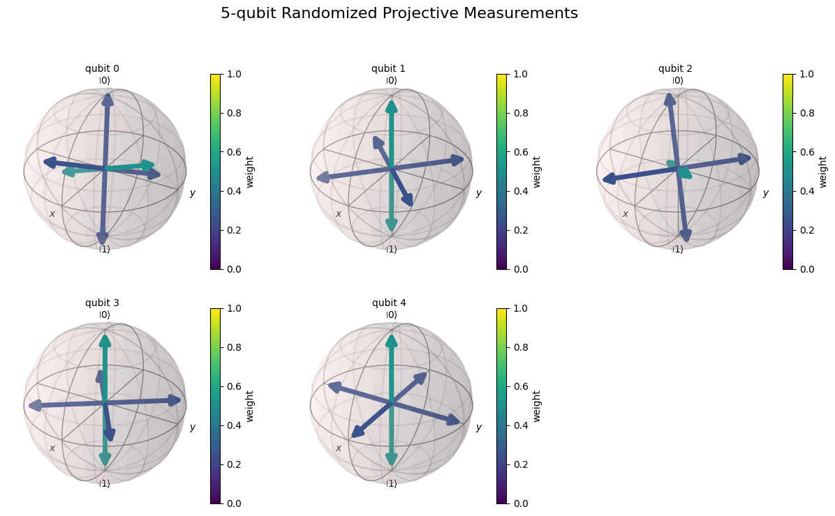
Define measurement procedure

import numpy as np
from numpy.random import default_rng
from povm_toolbox.library import RandomizedProjectiveMeasurements

rng = default_rng(96568)

num_qubits = qc.num_qubits

bias = np.array([0.5, 0.25, 0.25])
angles = np.array(
    [
        [2.01757238, -1.85001671, 2.52155716, 0.45636669, 1.17175533, -0.48263278],
        [0.0, 0.0, 1.57079633, -2.35619449, 1.57079633, -0.78539816],
        [1.94493547, -2.39620342, 0.3760775, -2.28966468, 1.53443501, 2.33046898],
        [0.0, 0.0, 1.57079633, 0.6, 1.57079633, 2.17079633],
        [0.0, 0.0, 1.57079633, 0.0, 1.57079633, 1.57079633],
    ]
)

measurement = RandomizedProjectiveMeasurements(num_qubits, bias=bias, angles=angles, seed_rng=rng)
measurement.definition().draw_bloch(
    title=f"{num_qubits}-qubit Randomized Projective Measurements", colorbar=True
)

Run the job

Initialize Sampler and POVMSampler. Then run the job.

from povm_toolbox.sampler import POVMSampler
from qiskit.primitives import StatevectorSampler

sampler = StatevectorSampler(seed=rng)
povm_sampler = POVMSampler(sampler=sampler)

job = povm_sampler.run([qc], shots=4096, povm=measurement)
pub_result = job.result()[0]

Define observable

from qiskit.quantum_info import SparsePauliOp

observable = SparsePauliOp(
    ["XIIII", "IIYII", num_qubits * "Y", num_qubits * "Z"], coeffs=[1.3, 1.2, -1, 1.4]
)

Choosing the dual frame

Given a POVM \(\{M_k\}_k\), a dual frame \(\{D_k\}_k\) can be obtained through

\[D_k = \frac{1}{\alpha_k}\mathcal{F}_{\alpha}^{-1}(M_k)\]

where the parametrized frame super-operator \(\mathcal{F}_{\alpha}\) is defined as

\[\mathcal{F}_{\alpha} : X \mapsto \sum_k \frac{\mathrm{Tr}[X M_k]}{\alpha_k} M_k\]

for parameters \(\{\alpha_k\}_k \subset \mathbb{R}\).

Canonical dual frame

The default case implemented in the POVMPostProcessor is to use the canonical dual frame, which is defined by parameters

\[\alpha_k = \mathrm{Tr}[M_k]\]

from povm_toolbox.post_processor import POVMPostProcessor
from qiskit.quantum_info import Statevector

exact_expectation_value = np.real_if_close(Statevector(qc).expectation_value(observable))
print(f"Exact value:     {exact_expectation_value}")

post_processor = POVMPostProcessor(pub_result)

exp_value_canonical, std_canonical = post_processor.get_expectation_value(observable)
print(f"Estimated value: {exp_value_canonical}")
print(f"\nEstimated standard deviation of the estimator: {std_canonical}")

Exact value:     0.9786732290044553
Estimated value: 0.7885807349016064

Estimated standard deviation of the estimator: 0.4044506732174399

State-marginal dual frame

Here we use the state-marginal dual frame, which requires the knowledge of the sampled state \(\rho\). More specifically, we compute the outcome probabilities

\[p_{k1,...,k_N} = \mathrm{Tr}[M_{k1,...,k_N} \rho]\]

where the POVM is assumed to have a product structure. We then marginalize these outcome probabilities to ensure that the dual frame will also have a product structure. That is, we set the parameters of the dual frame to

\[\alpha_{k1,...,k_N} = p^{(1)}_{k_1} \cdots p^{(N)}_{k_N}\]

where \(p^{(i)}_{k_i}\) is the (marginal) probability of obtaining outcome \(k_i\) on qubit \(i\).

The caveat of this dual frame is that we do not have access to the state \(\rho\) in general. However, it does work for testing and/or teaching purposes.

from povm_toolbox.post_processor import dual_from_marginal_probabilities

post_processor.dual = dual_from_marginal_probabilities(
    povm=post_processor.povm, state=Statevector(qc)
)

exp_value_marginal, std_marginal = post_processor.get_expectation_value(observable)
print(f"Estimated value: {exp_value_marginal}")
print(f"\nEstimated standard deviation of the estimator: {std_marginal}")

Estimated value: 0.9970974145287157

Estimated standard deviation of the estimator: 0.3041460424516805

Empirical frequencies dual frame

We now present a dual frame that uses the same idea as for the state-marginal dual frame, but without requiring the knowledge of the state \(\rho\) a priori. More precisely, we replace the marginal outcome probabilities by the empirical outcome frequencies:

\[\alpha_{k1,...,k_N} = f^{(1)}_{k_1} \cdots f^{(N)}_{k_N}\]

where \(f^{(i)}_{k_i} = \# k_i / S\) is the number of time we sampled outcome \(k_i\) on qubit \(i\) divided by the total number of shots \(S\).

To add stability of the estimator (and avoid parameters set to 0 if an outcome was not sampled), we add a bias term to the frequencies as

\[f^{(i)}_{k_i} = \frac{\# k_i + \mathrm{Tr}[\rho_{\mathrm{bias}} M^{(i)}_{k_i}] S_{\mathrm{bias}}}{S + S_{\mathrm{bias}}} \, ,\]

where \(\rho_{\mathrm{bias}}\) is an ansatz state (by default set to \(\frac{1}{d}\mathbb{I}\)) and \(S_{\mathrm{bias}}\) is the strength of the bias (by default set to the number of outcomes of the local POVM).

We have two edge cases: * In the limit \(S \to 0\), we recover the canonical dual frame if \(\rho_{\mathrm{bias}}=\frac{1}{d}\mathbb{I}\). * In the limit \(S \to \infty\), we recover the marginal-state dual frame (independently of \(\rho_{\mathrm{bias}}\)).

from povm_toolbox.post_processor import dual_from_empirical_frequencies

post_processor.dual = dual_from_empirical_frequencies(povm_post_processor=post_processor)

exp_value_freq, std_freq = post_processor.get_expectation_value(observable)
print(f"Estimated value: {exp_value_freq}")
print(f"\nEstimated standard deviation of the estimator: {std_freq}")

Estimated value: 1.0142327046854116

Estimated standard deviation of the estimator: 0.30334996039156614

Summary

We finally compare the estimates obtained with the different dual frames.

print(f"Exact value: {exact_expectation_value}\n")

print("Dual frame              Estimated value   Estimated std   Actual error")
print("------------------------------------------------------------------------")
print(
    f"canonical {exp_value_canonical:>29.6f} {std_canonical:>15.6f} {abs(exp_value_canonical - exact_expectation_value):>14.6f}"
)
print(
    f"marginal probabilities {exp_value_marginal:>16.6f} {std_marginal:>15.6f} {abs(exp_value_marginal - exact_expectation_value):>14.6f}"
)
print(
    f"empirical frequencies {exp_value_freq:>17.6f} {std_freq:>15.6f} {abs(exp_value_freq - exact_expectation_value):>14.6f}"
)

Exact value: 0.9786732290044553

Dual frame              Estimated value   Estimated std   Actual error
------------------------------------------------------------------------
canonical                      0.788581        0.404451       0.190092
marginal probabilities         0.997097        0.304146       0.018424
empirical frequencies          1.014233        0.303350       0.035559