Dilation POVMs and how to deal with ancilla qubits¶

This document shows you how to use dilation measurements. More specifically, it showcases how we deal with required measurement ancilla qubits.

[1]:

%load_ext autoreload
%autoreload 2

First example of a dilation POVM¶

[2]:

import numpy as np
from povm_toolbox.library import DilationMeasurements

# parameters that define a SIC-POVM (SIC stands for "symmetric and informationally-complete")
sic_parameters = np.array(
    [0.75, 0.30408673, 0.375, 0.40678524, 0.32509973, 0.25000035, 0.49999321, 0.83333313],
)

povm = DilationMeasurements(num_qubits=1, parameters=sic_parameters, insert_barriers=True)
povm.definition().draw_bloch()

[2]:

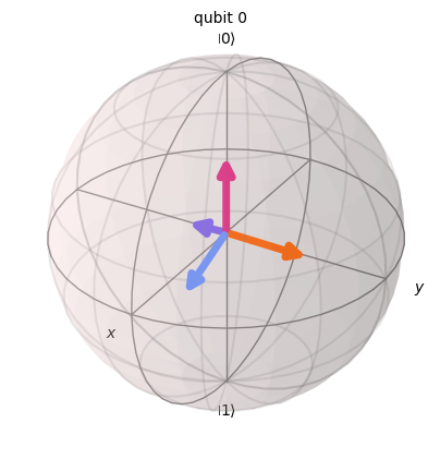
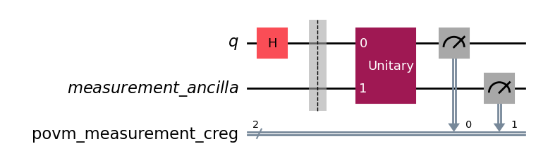
../_images/how_tos_dilation_measurements_3_0.png

IC dilation measurements are defined on a space spanning (at least) four states: e.g. \(\{|0\rangle,|1\rangle,|2\rangle,|3\rangle\}\). To achieve such a measurement using qubits, every qubit gets paired with an ancilla qubit. Then, the dilation measurement can be constructed via some two-qubit unitary followed by measurements in the computational basis. The binary outcomes \(\{|00\rangle,|01\rangle,|10\rangle,|11\rangle\}\) can then be mapped to the four states above.

[3]:

from qiskit.circuit import QuantumCircuit

qc = QuantumCircuit(1)
qc.h(0)

povm.compose_circuits(qc).draw("mpl")

[3]:

../_images/how_tos_dilation_measurements_5_0.png

Adding necessary ancilla qubits¶

The user doesn’t have to deal with adding ancilla qubits, the method DilationMeasurements.compose_circuit takes care of adding ancilla qubits when necessary. It will check if the input circuit has idling qubits that can be used. If there are not enough idling qubits in the input circuit, the method will add additional ancilla qubits to the input circuit.

1. Quantum Circuit without ancilla qubits¶

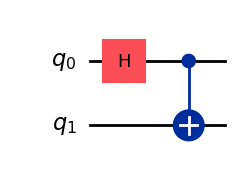
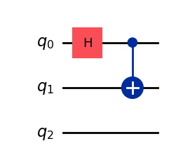
Example of a quantum circuit without idling qubits.

[4]:

qc = QuantumCircuit(2)
qc.h(0)
qc.cx(0, 1)

qc.draw("mpl")

[4]:

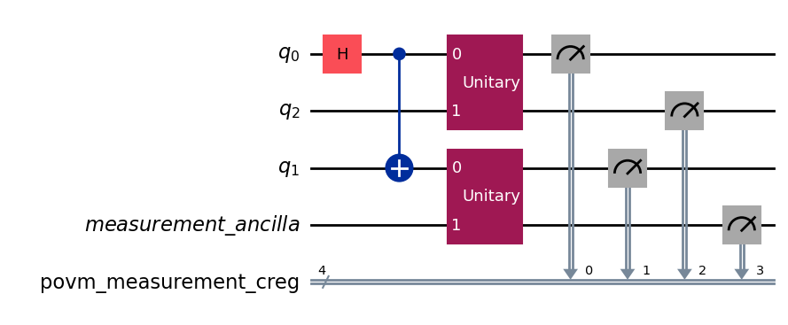
../_images/how_tos_dilation_measurements_8_0.png

[5]:

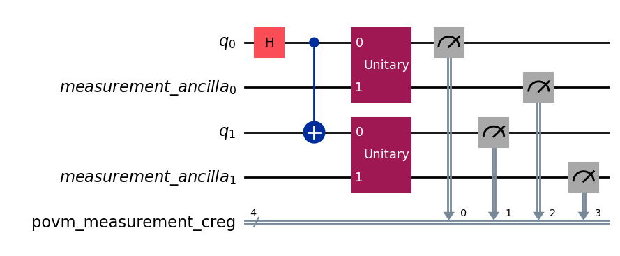
povm = DilationMeasurements(num_qubits=2, parameters=sic_parameters)

# The input circuit does not have any idling qubits. The method `compose_circuit` will add two ancilla qubits.
povm.compose_circuits(qc).draw("mpl", wire_order=[0, 2, 1, 3])

[5]:

../_images/how_tos_dilation_measurements_9_0.png

2. Quantum Circuit with a few idling qubits¶

Example of a quantum circuit with a few idling qubits, but not enough.

[6]:

qc = QuantumCircuit(3)
qc.h(0)
qc.cx(0, 1)

qc.draw("mpl")

[6]:

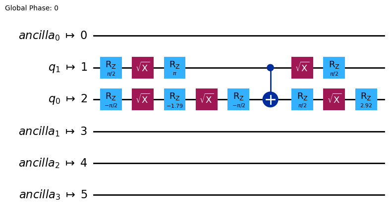
../_images/how_tos_dilation_measurements_11_0.png

[7]:

povm.measurement_layout = [0, 1]

# The input circuit has one idling qubit. The method `compose_circuit` will use it and also add one ancilla qubit.
povm.compose_circuits(qc).draw("mpl", wire_order=[0, 2, 1, 3])

[7]:

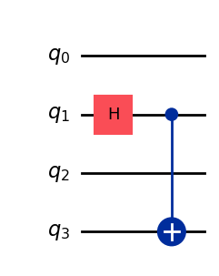
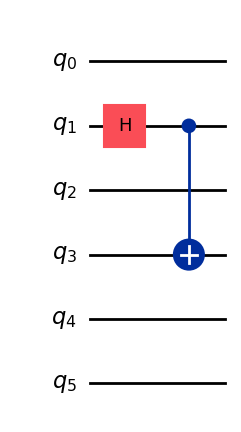
../_images/how_tos_dilation_measurements_12_0.png

3. Quantum Circuit with enough idling qubits¶

Example of a quantum circuit with enough idling qubits.

[8]:

qc = QuantumCircuit(4)
qc.h(1)
qc.cx(1, 3)

qc.draw("mpl")

[8]:

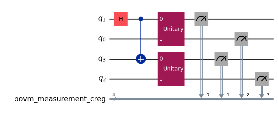
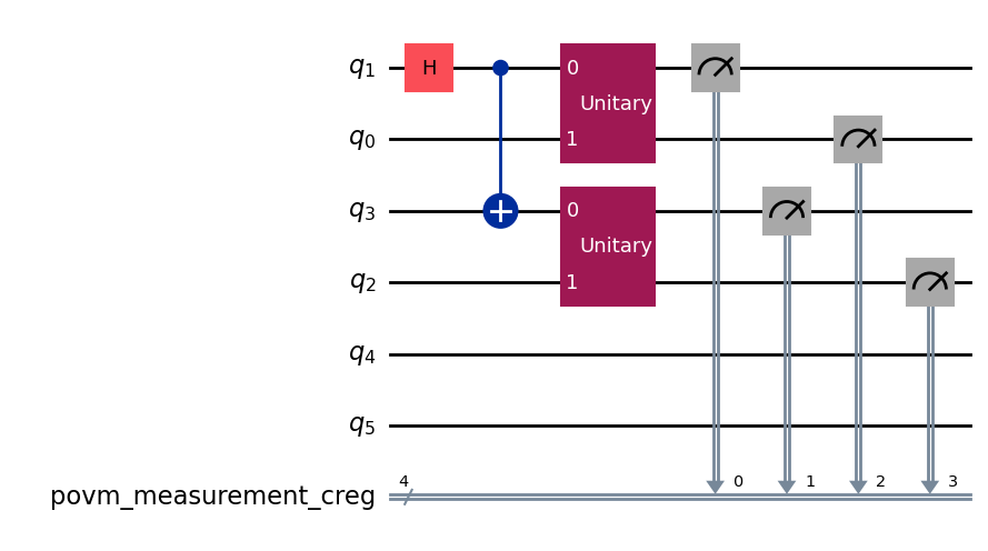
../_images/how_tos_dilation_measurements_14_0.png

[9]:

povm.measurement_layout = [1, 3]

# The input circuit has two idling qubit. The method `compose_circuit` will use both of them and does not need to add any additional ancilla qubits.
povm.compose_circuits(qc).draw("mpl", wire_order=[1, 0, 3, 2])

[9]:

../_images/how_tos_dilation_measurements_15_0.png

4. Quantum Circuit with many idling qubits¶

Example of a quantum circuit with more than enough idling qubits.

[10]:

qc = QuantumCircuit(6)
qc.h(1)
qc.cx(1, 3)

qc.draw("mpl")

[10]:

../_images/how_tos_dilation_measurements_17_0.png

[11]:

povm.measurement_layout = [1, 3]

# The input circuit has four idling qubit. The method `compose_circuit` will use two of them (and does not need to add any additional ancilla qubits).
povm.compose_circuits(qc).draw("mpl", wire_order=[1, 0, 3, 2, 4, 5])

[11]:

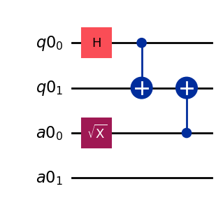
../_images/how_tos_dilation_measurements_18_0.png

5. Quantum circuit with ancilla qubits that are not idling¶

Example of a quantum circuit that has an AncillaRegister with non-idle qubits. These cannot be used and, thus, we need additional ancilla qubits to ensure all dilation measurements can be performed.

[12]:

from qiskit.circuit import AncillaRegister, QuantumRegister

qc = QuantumCircuit(QuantumRegister(2), AncillaRegister(2))
qc.h(0)
qc.cx(0, 1)
qc.sx(2)
qc.cx(2, 1)

qc.draw("mpl")

[12]:

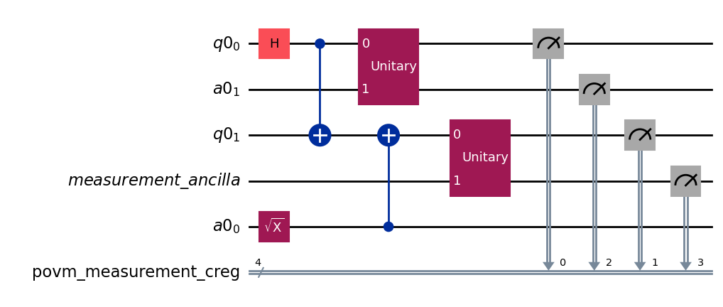
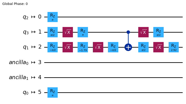
../_images/how_tos_dilation_measurements_20_0.png

[13]:

# We only want to measure qubits 0 and 1 (qubit 2 is an ancilla qubit)
povm.measurement_layout = [0, 1]

# The input circuit has one idling qubit. The method `compose_circuit` will use it and also add one ancilla qubit.
povm.compose_circuits(qc).draw("mpl", wire_order=[0, 3, 1, 4, 2])

[13]:

../_images/how_tos_dilation_measurements_21_0.png

Transpiled Quantum Circuits¶

Examples with transpiled quantum circuits.

Generate a generic backend¶

[14]:

from qiskit.providers.fake_provider import GenericBackendV2
from qiskit.transpiler.preset_passmanagers import generate_preset_pass_manager

# Generate a 6-qubit simulated backend
backend = GenericBackendV2(
    num_qubits=6, coupling_map=[[0, 2], [1, 2], [2, 3], [4, 3], [5, 3]], seed=0
)

backend.set_options(seed_simulator=25)
pm = generate_preset_pass_manager(optimization_level=2, backend=backend, seed_transpiler=0)

coupling_map = backend.coupling_map
# coupling_map.draw()

Define quantum circuit¶

[15]:

qc = QuantumCircuit(2)
qc.h(0)
qc.cx(0, 1)
qc.draw("mpl")

[15]:

../_images/how_tos_dilation_measurements_26_0.png

Transpile circuit¶

[16]:

# Transpile the circuit to an "Instruction Set Architecture" (ISA) circuit.
# Note: the transpiler automatically adds "ancilla" qubits to make the transpiled
# circuit match the size of the backend.
qc_isa = pm.run(qc)
qc_isa.draw("mpl")

[16]:

../_images/how_tos_dilation_measurements_28_0.png

Define measurement procedure¶

There is no need to set a particular measurement_layout, because the POVMSampler will analyze the transpiled circuit and apply the TranspileLayout to the measurement circuit.

[17]:

measurement = DilationMeasurements(
    num_qubits=2,
    parameters=sic_parameters,
    insert_barriers=True,
)

More precisely, the measurement layout that will be automatically applied by the POVMSampler is extracted as :

transpile_layout = transpiled_circuit.layout
measurement_layout = transpile_layout.final_index_layout(filter_ancillas=True)

For the above circuit, we have:

[18]:

print(qc_isa.layout.final_index_layout(filter_ancillas=True))

[2, 1]

Run the job¶

Initialize Sampler and POVMSampler. Then run the job. A pass manager has to be provided to transform the final composed circuit into an ISA circuit.

[19]:

from povm_toolbox.sampler import POVMSampler
from qiskit_ibm_runtime import SamplerV2 as RuntimeSampler

# First define a standard sampler (that will be used under the hood).
runtime_sampler = RuntimeSampler(mode=backend)
# Then define the POVM sampler, which takes the sampler as an argument.
povm_sampler = POVMSampler(runtime_sampler)
# Submit the job by specifying which POVM to use, which circuit(s) to measure and the shot budget.
# A pass manager has to be provided to make the measurement circuit ISA.
job = povm_sampler.run([qc_isa], shots=4096, povm=measurement, pass_manager=pm)

Look at the final composed circuit to check that the measurement was performed on the correct qubits. It is important to note that the two-qubit unitary which is part of the dilation measurement can cause a significant SWAP overhead, depending on the qubit connectivity between the measured qubit and its associated ancilla.

[20]:

pub_result = job.result()[0]
pub_result.metadata.composed_circuit.draw("mpl", fold=-1)

[20]:

../_images/how_tos_dilation_measurements_36_0.png

Define observable¶

[21]:

from qiskit.quantum_info import SparsePauliOp

observable = SparsePauliOp(["XI", "XX", "YY", "ZX"], coeffs=[1, 1, -1, 1])

Get the expected value¶

The observable has to be specified in terms of virtual qubits. Therefore, there is no need to apply the layout that was used by the POVM on the physical qubits.

[22]:

from povm_toolbox.post_processor import POVMPostProcessor

post_processor = POVMPostProcessor(pub_result)
exp_value, std = post_processor.get_expectation_value(observable)
print(exp_value)

2.0032563568087483

For reference, we can compare our estimated expectation value to the exact value.

[23]:

from qiskit.quantum_info import Statevector

isa_observable = observable.apply_layout(layout=qc_isa.layout, num_qubits=qc_isa.num_qubits)

exact_expectation_value = np.real_if_close(Statevector(qc_isa).expectation_value(isa_observable))
print(f"Exact value:     {exact_expectation_value}")
print(f"Estimated value: {exp_value}")

Exact value:     1.9999999999999987
Estimated value: 2.0032563568087483

Transpiled Quantum Circuit with ancilla qubits¶

Example where the quantum circuit had ancilla qubits before transpilation.

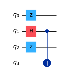
Define quantum circuit¶

The circuit can contain some ancilla qubits that you might not want to measure.

[24]:

qc_with_ancilla = QuantumCircuit(4)

# Qubits (1,3):
qc_with_ancilla.h(1)
qc_with_ancilla.cx(1, 3)

# Ancilla qubits (0,2):
qc_with_ancilla.z(0)
qc_with_ancilla.z(2)

qc_with_ancilla.draw("mpl")

[24]:

../_images/how_tos_dilation_measurements_45_0.png

Transpile circuit with ancilla qubits¶

[25]:

# Transpile the circuit to an "Instruction Set Architecture" (ISA) circuit
qc_with_ancilla_isa = pm.run(qc_with_ancilla)
qc_with_ancilla_isa.draw("mpl")

[25]:

../_images/how_tos_dilation_measurements_47_0.png

Define measurement procedure¶

The measurement_layout argument specifies which qubits to measure. This argument overrides the automatic detection of a possible TranspileLayout attribute of the supplied circuit. I.e., it specifies directly the (final) physical qubits on which the POVM will act. In this example, we want to measure physical qubits 4 and 3.

If you want to specify the virtual qubits instead (here virtual qubits 1 and 3), you have to do the composition with the TranspileLayout manually as follows:

[26]:

# Measuring virtual qubits 1 and 3
virtual_msmt_layout = [1, 3]
# Get the transpilation layout
transpile_layout = qc_with_ancilla_isa.layout.final_index_layout()
# Compute the final measurement layout
final_msmt_layout = [transpile_layout[idx] for idx in virtual_msmt_layout]
print("Final measurement layout:", final_msmt_layout)

measurement = DilationMeasurements(
    2,
    measurement_layout=final_msmt_layout,
    parameters=sic_parameters,
    insert_barriers=True,
)

Final measurement layout: [2, 1]

Run the job¶

Initialize Sampler and POVMSampler. Then run the job.

[27]:

# First define a standard sampler (that will be used under the hood).
runtime_sampler = RuntimeSampler(mode=backend)
# Then define the POVM sampler, which takes the sampler as an argument.
povm_sampler = POVMSampler(runtime_sampler)
# Submit the job by specifying which POVM to use, which circuit(s) to measure and the shot budget.
job = povm_sampler.run([qc_with_ancilla_isa], shots=4096, povm=measurement, pass_manager=pm)
pub_result = job.result()[0]

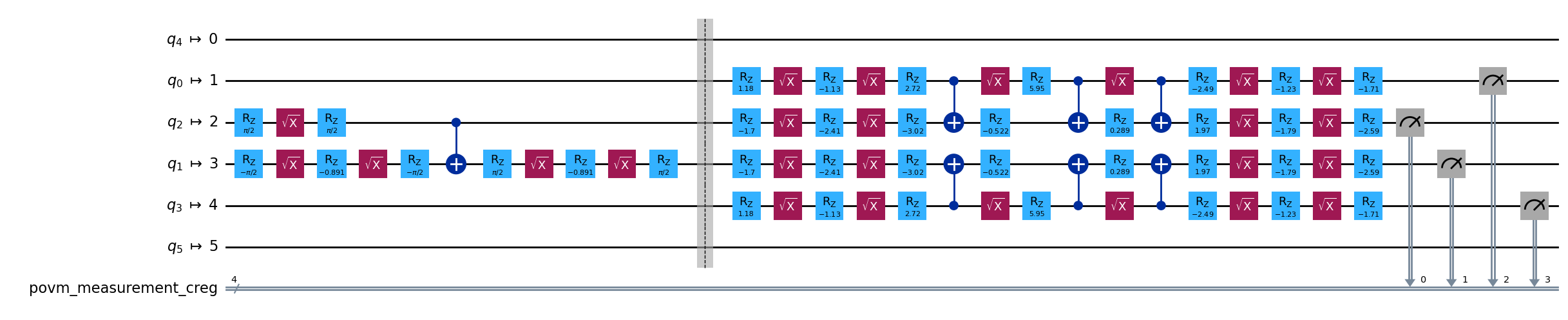
You can check that measurement was performed on the correct physical qubits by looking at the final composed circuit.

[28]:

pub_result.metadata.composed_circuit.draw("mpl", fold=-1)

[28]:

../_images/how_tos_dilation_measurements_53_0.png

Get the expected value¶

The observable has to be specified in terms of virtual qubits. Therefore, there is no need to apply the layout that was used by the POVM on the physical qubits.

[29]:

post_processor = POVMPostProcessor(pub_result)

print(f"Exact value:     {exact_expectation_value}")

exp_value, std = post_processor.get_expectation_value(observable)
print(f"Estimated value: {exp_value}")

Exact value:     1.9999999999999987
Estimated value: 2.0032563568087483