Quantum State Tomography¶

Quantum tomography is an experimental procedure to reconstruct a description of part of a quantum system from the measurement outcomes of a specific set of experiments. In particular, quantum state tomography reconstructs the density matrix of a quantum state by preparing the state many times and measuring them in a tomographically complete basis of measurement operators.

Note

This tutorial requires the qiskit-aer and qiskit-ibm-runtime packages to run simulations. You can install them with python -m pip install qiskit-aer qiskit-ibm-runtime.

We first initialize a simulator to run the experiments on.

from qiskit_aer import AerSimulator
from qiskit_ibm_runtime.fake_provider import FakePerth

backend = AerSimulator.from_backend(FakePerth())

To run a state tomography experiment, we initialize the experiment with a circuit to prepare the state to be measured. We can also pass in an Operator or a Statevector to describe the preparation circuit.

import qiskit
from qiskit_experiments.framework import ParallelExperiment
from qiskit_experiments.library import StateTomography

# GHZ State preparation circuit
nq = 2
qc_ghz = qiskit.QuantumCircuit(nq)
qc_ghz.h(0)
qc_ghz.s(0)
for i in range(1, nq):
    qc_ghz.cx(0, i)

# QST Experiment
qstexp1 = StateTomography(qc_ghz)
qstdata1 = qstexp1.run(backend, seed_simulation=100).block_for_results()

# Print results
display(qstdata1.analysis_results(dataframe=True))

	name	experiment	components	value	quality	backend	run_time	trace	eigvals	raw_eigvals	rescaled_psd	fitter_metadata	conditional_probability	positive
6c6a05c4	state	StateTomography	[Q0, Q1]	DensityMatrix([[ 0.45914714+0.j , 0.01...	None	aer_simulator_from(fake_perth)	None	1.0	[0.919198156377239, 0.04698324334911811, 0.028...	[0.919198156377239, 0.04698324334911811, 0.028...	False	{'fitter': 'linear_inversion', 'fitter_time': ...	1.0	True
469d0d48	state_fidelity	StateTomography	[Q0, Q1]	0.918457	None	aer_simulator_from(fake_perth)	None	None	None	None	None	None	None	None
6204da39	positive	StateTomography	[Q0, Q1]	True	None	aer_simulator_from(fake_perth)	None	None	None	None	None	None	None	None

Tomography Results¶

The main result for tomography is the fitted state, which is stored as a DensityMatrix object:

state_result = qstdata1.analysis_results("state", dataframe=True).iloc[0]
print(state_result.value)

DensityMatrix([[ 0.45914714+0.j        ,  0.01025391-0.0086263j ,
                 0.00927734+0.00276693j, -0.01318359-0.44921875j],
               [ 0.01025391+0.0086263j ,  0.03011068+0.j        ,
                -0.01318359+0.j        , -0.01123047-0.00406901j],
               [ 0.00927734-0.00276693j, -0.01318359+0.j        ,
                 0.03141276+0.j        , -0.00830078-0.01155599j],
               [-0.01318359+0.44921875j, -0.01123047+0.00406901j,
                -0.00830078+0.01155599j,  0.47932943+0.j        ]],
              dims=(2, 2))

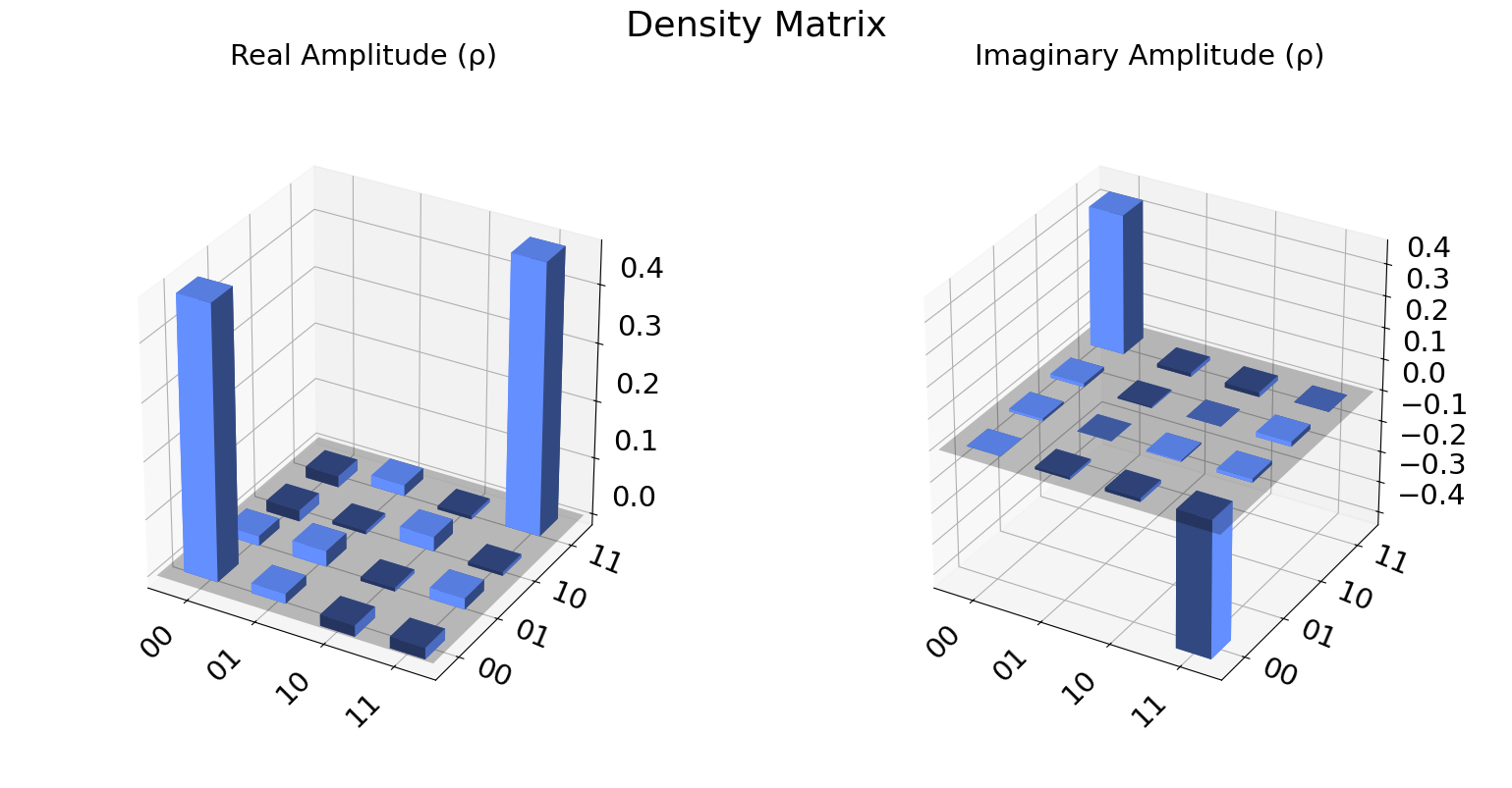
We can also visualize the density matrix:

from qiskit.visualization import plot_state_city
state = qstdata1.analysis_results("state", dataframe=True).iloc[0].value
plot_state_city(state, title='Density Matrix')

The state fidelity of the fitted state with the ideal state prepared by the input circuit is stored in the "state_fidelity" result field. Note that if the input circuit contained any measurements the ideal state cannot be automatically generated and this field will be set to None.

fid_result = qstdata1.analysis_results("state_fidelity", dataframe=True).iloc[0]
print("State Fidelity = {:.5f}".format(fid_result.value))

State Fidelity = 0.91846

Additional state metadata¶

Additional data is stored in the tomography under additional fields. This includes

eigvals: the eigenvalues of the fitted state
trace: the trace of the fitted state
positive: Whether the eigenvalues are all non-negative

If trace rescaling was performed this dictionary will also contain a raw_trace field containing the trace before rescaling. Futhermore, if the state was rescaled to be positive or trace 1 an additional field raw_eigvals will contain the state eigenvalues before rescaling was performed.

for col in ["eigvals", "trace", "positive"]:
    print(f"{col}: {state_result[col]}")

eigvals: [0.91919816 0.04698324 0.02892367 0.00489493]
trace: 1.000000000000001
positive: True

To see the effect of rescaling, we can perform a “bad” fit with very low counts:

# QST Experiment
bad_data = qstexp1.run(backend, shots=10, seed_simulation=100).block_for_results()
bad_state_result = bad_data.analysis_results("state", dataframe=True).iloc[0]

# Print result
for key, val in bad_state_result.items():
    print(f"{key}: {val}")

name: state
experiment: StateTomography
components: [<Qubit(Q0)>, <Qubit(Q1)>]
value: DensityMatrix([[ 0.43608661+0.00000000e+00j,  0.09545365+1.29166135e-02j,
                -0.03688001+7.32474804e-02j,  0.00646826-3.49857117e-01j],
               [ 0.09545365-1.29166135e-02j,  0.03542661+0.00000000e+00j,
                -0.00897047+9.70260775e-03j,  0.03263655-1.00678478e-01j],
               [-0.03688001-7.32474804e-02j, -0.00897047-9.70260775e-03j,
                 0.02861705+0.00000000e+00j, -0.07299639+4.16493120e-02j],
               [ 0.00646826+3.49857117e-01j,  0.03263655+1.00678478e-01j,
                -0.07299639-4.16493120e-02j,  0.49986973-6.93889390e-18j]],
              dims=(2, 2))
quality: None
backend: aer_simulator_from(fake_perth)
run_time: None
trace: 1.0000000000000009
eigvals: [0.86026194 0.12496074 0.01477732 0.        ]
raw_eigvals: [ 0.89891231  0.16361111  0.05342768 -0.1159511 ]
rescaled_psd: True
fitter_metadata: {'fitter': 'linear_inversion', 'fitter_time': 0.0039331912994384766}
conditional_probability: 1.0
positive: True

Tomography Fitters¶

The default fitters is linear_inversion, which reconstructs the state using dual basis of the tomography basis. This will typically result in a non-positive reconstructed state. This state is rescaled to be positive-semidefinite (PSD) by computing its eigen-decomposition and rescaling its eigenvalues using the approach from Ref. [1].

There are several other fitters are included (See API documentation for details). For example, if cvxpy is installed we can use the cvxpy_gaussian_lstsq() fitter, which allows constraining the fit to be PSD without requiring rescaling.

try:
    import cvxpy

    # Set analysis option for cvxpy fitter
    qstexp1.analysis.set_options(fitter='cvxpy_gaussian_lstsq')

    # Re-run experiment
    qstdata2 = qstexp1.run(backend, seed_simulation=100).block_for_results()

    state_result2 = qstdata2.analysis_results("state", dataframe=True).iloc[0]
    for key, val in state_result2.items():
        print(f"{key}: {val}")

except ModuleNotFoundError:
    print("CVXPY is not installed")

name: state
experiment: StateTomography
components: [<Qubit(Q0)>, <Qubit(Q1)>]
value: DensityMatrix([[ 4.77385497e-01+0.j        ,  9.13079993e-03-0.01134232j,
                 8.33375234e-03+0.0031693j , -1.51344600e-02-0.44016457j],
               [ 9.13079993e-03+0.01134232j,  3.51646408e-02+0.j        ,
                -1.80746266e-02+0.00279125j, -3.66068786e-03-0.00364678j],
               [ 8.33375234e-03-0.0031693j , -1.80746266e-02-0.00279125j,
                 2.21091687e-02+0.j        ,  3.65148367e-04+0.00783394j],
               [-1.51344600e-02+0.44016457j, -3.66068786e-03+0.00364678j,
                 3.65148367e-04-0.00783394j,  4.65340694e-01+0.j        ]],
              dims=(2, 2))
quality: None
backend: aer_simulator_from(fake_perth)
run_time: None
trace: 1.000000002034044
eigvals: [0.91196631 0.05425153 0.0300069  0.00377526]
raw_eigvals: [0.91196631 0.05425153 0.0300069  0.00377526]
rescaled_psd: False
fitter_metadata: {'fitter': 'cvxpy_gaussian_lstsq', 'cvxpy_solver': 'SCS', 'cvxpy_status': ['optimal'], 'psd_constraint': True, 'trace_preserving': True, 'fitter_time': 0.03258657455444336}
conditional_probability: 1.0
positive: True

Parallel Tomography Experiment¶

We can also use the ParallelExperiment class to run subsystem tomography on multiple qubits in parallel.

For example if we want to perform 1-qubit QST on several qubits at once:

from math import pi
num_qubits = 5
gates = [qiskit.circuit.library.RXGate(i * pi / (num_qubits - 1))
         for i in range(num_qubits)]

subexps = [
    StateTomography(gate, physical_qubits=(i,))
    for i, gate in enumerate(gates)
]
parexp = ParallelExperiment(subexps)
pardata = parexp.run(backend, seed_simulation=100).block_for_results()

display(pardata.analysis_results(dataframe=True))

	name	experiment	components	value	quality	backend	run_time	trace	eigvals	raw_eigvals	rescaled_psd	fitter_metadata	conditional_probability	positive
caea0fe6	state	StateTomography	[Q0]	DensityMatrix([[ 0.96972656+0.j , -0.00...	None	aer_simulator_from(fake_perth)	None	1.0	[0.9697681813033308, 0.03023181869667016]	[0.9697681813033308, 0.03023181869667016]	False	{'fitter': 'linear_inversion', 'fitter_time': ...	1.0	True
f849e946	state_fidelity	StateTomography	[Q0]	0.969727	None	aer_simulator_from(fake_perth)	None	None	None	None	None	None	None	None
4e995942	positive	StateTomography	[Q0]	True	None	aer_simulator_from(fake_perth)	None	None	None	None	None	None	None	None
8c824478	state	StateTomography	[Q1]	DensityMatrix([[0.86262789+0.j , 0.0048...	None	aer_simulator_from(fake_perth)	None	1.0	[1.0000000000000009, 0.0]	[1.0035938802891162, -0.0035938802891152255]	True	{'fitter': 'linear_inversion', 'fitter_time': ...	1.0	True
4bcfb943	state_fidelity	StateTomography	[Q1]	0.999807	None	aer_simulator_from(fake_perth)	None	None	None	None	None	None	None	None
60e90429	positive	StateTomography	[Q1]	True	None	aer_simulator_from(fake_perth)	None	None	None	None	None	None	None	None
ae0904dd	state	StateTomography	[Q2]	DensityMatrix([[ 0.51171875+0.j , -0.01...	None	aer_simulator_from(fake_perth)	None	1.0	[0.9720232800060566, 0.02797671999394402]	[0.9720232800060566, 0.02797671999394402]	False	{'fitter': 'linear_inversion', 'fitter_time': ...	1.0	True
9b20b01c	state_fidelity	StateTomography	[Q2]	0.97168	None	aer_simulator_from(fake_perth)	None	None	None	None	None	None	None	None
f12ab20d	positive	StateTomography	[Q2]	True	None	aer_simulator_from(fake_perth)	None	None	None	None	None	None	None	None
a1fc0e73	state	StateTomography	[Q3]	DensityMatrix([[ 0.14453125+0.j , -0.006...	None	aer_simulator_from(fake_perth)	None	1.0	[0.9891408449253822, 0.010859155074618987]	[0.9891408449253822, 0.010859155074618987]	False	{'fitter': 'linear_inversion', 'fitter_time': ...	1.0	True
bac92e1e	state_fidelity	StateTomography	[Q3]	0.988898	None	aer_simulator_from(fake_perth)	None	None	None	None	None	None	None	None
0a945e02	positive	StateTomography	[Q3]	True	None	aer_simulator_from(fake_perth)	None	None	None	None	None	None	None	None
c54dc0d2	state	StateTomography	[Q4]	DensityMatrix([[0.03125 +0.j , 0.0253...	None	aer_simulator_from(fake_perth)	None	1.0	[0.9695387244621378, 0.030461275537863288]	[0.9695387244621378, 0.030461275537863288]	False	{'fitter': 'linear_inversion', 'fitter_time': ...	1.0	True
420aa95b	state_fidelity	StateTomography	[Q4]	0.96875	None	aer_simulator_from(fake_perth)	None	None	None	None	None	None	None	None
959f5349	positive	StateTomography	[Q4]	True	None	aer_simulator_from(fake_perth)	None	None	None	None	None	None	None	None

View experiment analysis results for one component:

results = pardata.analysis_results(dataframe=True)
display(results[results.components.apply(lambda x: x == ["Q0"])])

	name	experiment	components	value	quality	backend	run_time	trace	eigvals	raw_eigvals	rescaled_psd	fitter_metadata	conditional_probability	positive
caea0fe6	state	StateTomography	[Q0]	DensityMatrix([[ 0.96972656+0.j , -0.00...	None	aer_simulator_from(fake_perth)	None	1.0	[0.9697681813033308, 0.03023181869667016]	[0.9697681813033308, 0.03023181869667016]	False	{'fitter': 'linear_inversion', 'fitter_time': ...	1.0	True
f849e946	state_fidelity	StateTomography	[Q0]	0.969727	None	aer_simulator_from(fake_perth)	None	None	None	None	None	None	None	None
4e995942	positive	StateTomography	[Q0]	True	None	aer_simulator_from(fake_perth)	None	None	None	None	None	None	None	None

Quantum State Tomography¶

Tomography Results¶

Additional state metadata¶

Tomography Fitters¶

Parallel Tomography Experiment¶

References¶

See also¶