Data Processor: Wrangling data

Data processing is the act of taking the data returned by the backend and converting it into a format that can be analyzed. It is implemented as a chain of data processing steps that transform various input data, e.g. IQ data, into a desired format, e.g. population, which can be analyzed. These data transformations may consist of multiple steps, such as kerneling and discrimination. Each step is implemented by a member of the DataAction class, also called a node.

The data processor implements the __call__() method. Once initialized, it can thus be used as a standard python function:

processor = DataProcessor(input_key="memory", [Node1(), Node2(), ...])
out_data = processor(in_data)

The data input to the processor is a sequence of dictionaries each representing the result of a single circuit. The output of the processor is a numpy array whose shape and data type depend on the combination of the nodes in the data processor.

Uncertainties that arise from quantum measurements or finite sampling can be taken into account in the nodes: a standard error can be generated in a node and can be propagated through the subsequent nodes in the data processor. Correlation between computed values is also considered.

Let’s look at an example to see how to initialize an instance of DataProcessor and create the DataAction nodes that process the data.

Data types on IBM Quantum backends

IBM Quantum backends can return different types of data. There is counts data and IQ data [1], referred to as level 2 and level 1 data, respectively. Level 2 data corresponds to a dictionary with bit-strings as keys and the number of times the bit-string was measured as a value. Importantly for some experiments, the backends can return a lower data level known as IQ data. Here, I and Q stand for in phase and quadrature. The IQ are points in the complex plane corresponding to a time integrated measurement signal which is reflected or transmitted through the readout resonator depending on the setup. IQ data can be returned as “single” or “averaged” data. Here, single means that the outcome of each single shot is returned while average only returns the average of the IQ points over the measured shots. The type of data that an experiment should return is specified by the run_options() of an experiment.

Processing data of different types

An experiment should work with the different data levels. Crucially, the analysis, such as a curve analysis, expects the same data format no matter the run options of the experiment. Transforming the data returned by the backend into the format that the analysis accepts is done by the data_processing library. The key class here is the DataProcessor. It is initialized from two arguments. The first is the input_key, which is typically “memory” or “counts”, and identifies the key in the experiment data where the data is located. The second argument data_actions is a list of nodes where each node performs a processing step of the data processor. Crucially, the output of one node in the list is the input to the next node in the list.

To illustrate the data processing module, we consider an example in which we measure a rabi oscillation with different data levels. The code below sets up the Rabi experiment.

Note

This tutorial requires the qiskit_dynamics package to run simulations. You can install it with python -m pip install qiskit-dynamics.

import numpy as np

from qiskit import pulse
from qiskit.circuit import Parameter

from qiskit_experiments.test.pulse_backend import SingleTransmonTestBackend
from qiskit_experiments.data_processing import DataProcessor, nodes
from qiskit_experiments.library import Rabi

with pulse.build() as sched:
    pulse.play(
        pulse.Gaussian(160, Parameter("amp"), sigma=40),
        pulse.DriveChannel(0)
    )

backend = SingleTransmonTestBackend(seed=100)

exp = Rabi(
    physical_qubits=(0,),
    backend=backend,
    schedule=sched,
    amplitudes=np.linspace(-0.1, 0.1, 21)
)

We now run the Rabi experiment twice, once with level 1 data and once with level 2 data. Here, we manually configure two data processors but note that typically you do not need to do this yourself. We begin with single-shot IQ data.

data_nodes = [nodes.SVD(), nodes.AverageData(axis=1), nodes.MinMaxNormalize()]
iq_processor = DataProcessor("memory", data_nodes)
exp.analysis.set_options(data_processor=iq_processor)

exp_data = exp.run(meas_level=1, meas_return="single").block_for_results()

display(exp_data.figure(0))

Since we requested IQ data we set the input key to “memory” which is the key under which the data is located in the experiment data. The iq_processor contains three nodes. The first node SVD is a singular value decomposition which projects the two-dimensional IQ data on its main axis. The second node averages the single-shot data. The output is a single float per quantum circuit. Finally, the last node MinMaxNormalize normalizes the measured signal to the interval [0, 1]. 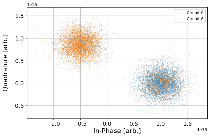The iq_dataprocessor is then set as an option of the analysis class. For those who are wondering what single-shot IQ data looks like we plot the data returned by the zeroth and sixth circuit in the code block below.

from qiskit_experiments.visualization import IQPlotter, MplDrawer

plotter = IQPlotter(MplDrawer())

for idx in [0, 6]:
    plotter.set_series_data(
        f"Circuit {idx}",
        points=np.array(exp_data.data(idx)["memory"]).squeeze(),
    )

plotter.figure()

Now we turn to counts data and see how the data processor needs to be changed.

data_nodes = [nodes.Probability(outcome="1")]
count_processor = DataProcessor("counts", data_nodes)
exp.analysis.set_options(data_processor=count_processor)

exp_data = exp.run(meas_level=2).block_for_results()

display(exp_data.figure(0))

Now, the input_key is “counts” since that is the key under which the counts data is saved in instances of ExperimentData. The list of nodes comprises a single data action which converts the counts to an estimation of the probability of measuring the outcome “1”.

Writing data actions

The nodes in a data processor are all sub-classes of DataAction. Users who wish to write their own data actions must (i) sub-class DataAction and (ii) implement the internal _process method called by instances of DataProcessor. This method is the processing step that the node implements. It takes a numpy array as input and returns the processed numpy array as output. This output serves as the input for the next node in the data processing chain. Here, the input and output numpy arrays can have a different shape.

In addition to the standard DataAction the data processing package also supports trainable data actions as subclasses of TrainableDataAction. These nodes must first be trained on the data before they can process the data. An example of a TrainableDataAction is the SVD node which must first learn the main axis of the data before it can project a data point onto this axis. To implement trainable nodes developers must also implement the train() method. This method is called when train() is called.

Conclusion

Data is processed by data processors that call a list of nodes each acting once on the data. Data processing connects the data returned by the backend to the data that the analysis classes need. Typically, you will not need to implement the data processing yourself since Qiskit Experiments has built-in methods that determine the correct instance of DataProcessor for your data. More advanced data processing includes, for example, handling restless measurements.

References

[1]

Thomas Alexander, Naoki Kanazawa, Daniel J. Egger, Lauren Capelluto, Christopher J. Wood, Ali Javadi-Abhari, David McKay, Qiskit Pulse: Programming Quantum Computers Through the Cloud with Pulses, Quantum Science and Technology 5, 044006 (2020). https://arxiv.org/abs/2004.06755.

See also

• Experiment manual: Restless Measurements