Randomized Benchmarking

Randomized benchmarking (RB) is a popular protocol for characterizing the error rate of quantum processors. An RB experiment consists of the generation of random Clifford circuits on the given qubits such that the unitary computed by the circuits is the identity. After running the circuits, the number of shots resulting in an error (i.e. an output different from the ground state) are counted, and from this data one can infer error estimates for the quantum device, by calculating the Error Per Clifford. See the Qiskit Textbook for an explanation on the RB method, which is based on Refs. [1] [2].

Note

This tutorial requires the qiskit-aer package to run simulations. You can install it with python -m pip install qiskit-aer.

import numpy as np
from qiskit_experiments.library import StandardRB, InterleavedRB
from qiskit_experiments.framework import ParallelExperiment, BatchExperiment
import qiskit.circuit.library as circuits

# For simulation
from qiskit_aer import AerSimulator
from qiskit_aer.noise import NoiseModel, depolarizing_error

noise_model = NoiseModel()
noise_model.add_all_qubit_quantum_error(depolarizing_error(5e-3, 1), ["sx", "x"])
noise_model.add_all_qubit_quantum_error(depolarizing_error(0, 1), ["rz"])
noise_model.add_all_qubit_quantum_error(depolarizing_error(5e-2, 2), ["cx"])
backend = AerSimulator(noise_model=noise_model)

Standard RB experiment

To run the RB experiment we need to provide the following RB parameters, in order to generate the RB circuits and run them on a backend:

• qubits: The number of qubits or list of physical qubits for the experiment

• lengths: A list of RB sequences lengths

• num_samples: Number of samples to generate for each sequence length

• seed: Seed or generator object for random number generation. If None then default_rng will be used

• full_sampling: If True all Cliffords are independently sampled for all lengths. If False for sample of lengths longer sequences are constructed by appending additional Clifford samples to shorter sequences. The default is False

Note

In the examples here, the sequence lengths and number of samples are chosen to be as low as possible while still producing typical results in order to minimize the simulation times. For accurate results, larger numbers may be necessary.

The analysis results of the RB Experiment may include:

• EPC: The estimated Error Per Clifford

• alpha: The depolarizing parameter. The fitting function is \(a \cdot \alpha^m + b\), where \(m\) is the Clifford length

• EPG: The Error Per Gate calculated from the EPC, only for 1-qubit or 2-qubit quantum gates (see [3])

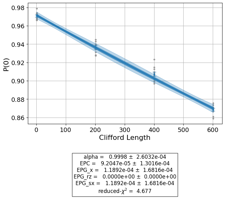
Running a 1-qubit RB experiment

The standard RB experiment will provide you gate errors for every basis gate constituting an averaged Clifford gate. Note that you can only obtain a single EPC value \(\cal E\) from a single RB experiment. As such, computing the error values for multiple gates \(\{g_i\}\) requires some assumption of contribution of each gate to the total depolarizing error. This is provided by the gate_error_ratio analysis option.

Provided that we have \(n_i\) gates with independent error \(e_i\) per Clifford, the total EPC is estimated by the composition of error from every basis gate,

\[{\cal E} = 1 - \prod_{i} (1 - e_i)^{n_i} \sim \sum_{i} n_i e_i + O(e^2),\]

where \(e_i \ll 1\) and the higher order terms can be ignored.

We cannot distinguish \(e_i\) with a single EPC value \(\cal E\) as explained, however by defining an error ratio \(r_i\) with respect to some standard value \(e_0\), we can compute EPG \(e_i\) for each basis gate.

\[{\cal E} \sim e_0 \sum_{i} n_i r_i\]

The EPG of the \(i\) th basis gate will be

\[e_i \sim r_i e_0 = \dfrac{r_i{\cal E}}{\sum_{i} n_i r_i}.\]

Because EPGs are computed based on this simple assumption, this is not necessarily representing the true gate error on the hardware. If you have multiple kinds of basis gates with unclear error ratio \(r_i\), interleaved RB experiment will always give you accurate error value \(e_i\).

lengths = [1, 10, 30, 80, 150] + np.arange(200, 1100, 200).tolist()
num_samples = 5
seed = 1010
qubits = [0]

# Run an RB experiment on qubit 0
exp1 = StandardRB(qubits, lengths, num_samples=num_samples, seed=seed)
expdata1 = exp1.run(backend).block_for_results()

# View result data
print("Gate error ratio: %s" % expdata1.experiment.analysis.options.gate_error_ratio)
display(expdata1.figure(0))
display(expdata1.analysis_results(dataframe=True))

Gate error ratio: {'x': 1.0, 'rz': 0.0, 'sx': 1.0}

	name	experiment	components	value	quality	backend	run_time	chisq
e807e042	alpha	StandardRB	[Q0]	0.99594+/-0.00008	good	aer_simulator	None	0.811461
4d8ff54b	EPC	StandardRB	[Q0]	0.00203+/-0.00004	good	aer_simulator	None	0.811461
28e323bc	EPG_x	StandardRB	[Q0]	0.00238+/-0.00005	good	aer_simulator	None	0.811461
9843e1e2	EPG_rz	StandardRB	[Q0]	0.0+/-0	good	aer_simulator	None	0.811461
e85d6d4c	EPG_sx	StandardRB	[Q0]	0.00238+/-0.00005	good	aer_simulator	None	0.811461

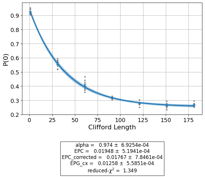
Running a 2-qubit RB experiment

In the same way we can compute EPC for two-qubit RB experiment. However, the EPC value obtained by the experiment indicates a depolarization which is a composition of underlying error channels for 2Q gates and 1Q gates in each qubit. Usually 1Q gate contribution is small enough to ignore, but in case this contribution is significant comparing to the 2Q gate error, we can decompose the contribution of 1Q gates [3].

\[\alpha_{2Q,C} = \frac{1}{5} \left( \alpha_0^{N_1/2} + \alpha_1^{N_1/2} + 3 \alpha_0^{N_1/2} \alpha_1^{N_1/2} \right) \alpha_{01}^{N_2},\]

where \(\alpha_i\) is the single qubit depolarizing parameter of channel \(i\), and \(\alpha_{01}\) is the two qubit depolarizing parameter of interest. \(N_1\) and \(N_2\) are total count of single and two qubit gates, respectively.

Note that the single qubit gate sequence in the channel \(i\) may consist of multiple kinds of basis gates \(\{g_{ij}\}\) with different EPG \(e_{ij}\). Therefore the \(\alpha_i^{N_1/2}\) should be computed from EPGs, rather than directly using the \(\alpha_i\), which is usually a composition of depolarizing maps of every single qubit gate. As such, EPGs should be measured in the separate single-qubit RBs in advance.

\[\alpha_i^{N_1/2} = \alpha_{i0}^{n_{i0}} \cdot \alpha_{i1}^{n_{i1}} \cdot ...,\]

where \(\alpha_{ij}^{n_{ij}}\) indicates a depolarization due to a particular basis gate \(j\) in the channel \(i\). Here we assume EPG \(e_{ij}\) corresponds to the depolarizing probability of the map of \(g_{ij}\), and thus we can express \(\alpha_{ij}\) with EPG.

\[e_{ij} = \frac{2^n - 1}{2^n} (1 - \alpha_{ij}) = \frac{1 - \alpha_{ij}}{2},\]

for the single qubit channel \(n=1\). Accordingly,

\[\alpha_i^{N_1/2} = \prod_{j} (1 - 2 e_{ij})^{n_{ij}},\]

as a composition of depolarization from every primitive gates per qubit. This correction will give you two EPC values as a result of the two-qubit RB experiment. The corrected EPC must be closer to the outcome of interleaved RB. The EPGs of two-qubit RB are analyzed with the corrected EPC if available.

lengths_2_qubit = np.arange(1, 80, 10)
lengths_1_qubit = [1, 10, 30, 80, 150] + np.arange(200, 1100, 200).tolist()
num_samples = 5
seed = 1010
qubits = (1, 2)

# Run a 1-qubit RB experiment on qubits 1, 2 to determine the error-per-gate of 1-qubit gates
single_exps = BatchExperiment(
    [
        StandardRB((qubit,), lengths_1_qubit, num_samples=num_samples, seed=seed)
        for qubit in qubits
    ]
)
expdata_1q = single_exps.run(backend).block_for_results()

# Run an RB experiment on qubits 1, 2
exp_2q = StandardRB(qubits, lengths_2_qubit, num_samples=num_samples, seed=seed)

# Use the EPG data of the 1-qubit runs to ensure correct 2-qubit EPG computation
exp_2q.analysis.set_options(epg_1_qubit=expdata_1q.analysis_results(dataframe=True))

# Run the 2-qubit experiment
expdata_2q = exp_2q.run(backend).block_for_results()

# View result data
print("Gate error ratio: %s" % expdata_2q.experiment.analysis.options.gate_error_ratio)
display(expdata_2q.figure(0))
display(expdata_2q.analysis_results(dataframe=True))

Gate error ratio: {'cx': 1.0}

	name	experiment	components	value	quality	backend	run_time	chisq
9f53fdee	alpha	StandardRB	[Q1, Q2]	0.9185+/-0.0035	bad	aer_simulator	None	4.271786
62b6b420	EPC	StandardRB	[Q1, Q2]	0.0611+/-0.0026	bad	aer_simulator	None	4.271786
e8577b5f	EPC_corrected	StandardRB	[Q1, Q2]	0.0530+/-0.0027	bad	aer_simulator	None	4.271786
027c85f4	EPG_cx	StandardRB	[Q1, Q2]	0.0352+/-0.0018	bad	aer_simulator	None	4.271786

Note that EPC_corrected value is smaller than one of raw EPC, which indicates contribution of depolarization from single-qubit error channels. If you don’t need EPG value, you can skip its computation by exp_2q.analysis.set_options(gate_error_ratio=False).

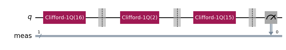
Displaying the RB circuits

The default RB circuit output shows Clifford blocks:

# Run an RB experiment on qubit 0
exp = StandardRB(physical_qubits=(0,), lengths=[2], num_samples=1, seed=seed)
c = exp.circuits()[0]
c.draw(output="mpl", style="iqp")

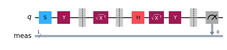
You can decompose the circuit into underlying gates:

c.decompose().draw(output="mpl", style="iqp")

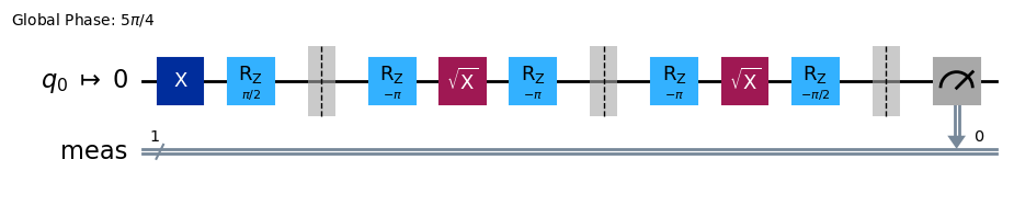
And see the transpiled circuit using the basis gate set of the backend:

from qiskit import transpile
transpile(c, backend, **vars(exp.transpile_options)).draw(output="mpl", style="iqp", idle_wires=False)

Note

In 0.5.0, the default value of optimization_level in transpile_options changed from 0 to 1 for RB experiments. Transpiled circuits may have less number of gates after the change.

Interleaved RB experiment

The interleaved RB experiment is used to estimate the gate error of the interleaved gate (see [4]). In addition to the usual RB parameters, we also need to provide:

• interleaved_element: the element to interleave, given either as a group element or as an instruction/circuit

The analysis results of the RB Experiment includes the following:

• EPC: The estimated error of the interleaved gate

• alpha and alpha_c: The depolarizing parameters of the original and interleaved RB sequences respectively

Extra analysis results include

• EPC_systematic_err: The systematic error of the interleaved gate error [4]

• EPC_systematic_bounds: The systematic error bounds of the interleaved gate error [4]

Let’s run an interleaved RB experiment on two qubits:

lengths = [1, 2, 4, 8] + np.arange(10, 80, 10).tolist()
num_samples = 3
seed = 1010
qubits = (1, 2)

# The interleaved gate is the CX gate
int_exp2 = InterleavedRB(
    circuits.CXGate(), qubits, lengths, num_samples=num_samples, seed=seed)

int_expdata2 = int_exp2.run(backend).block_for_results()
int_results2 = int_expdata2.analysis_results(dataframe=True)

# View result data
display(int_expdata2.figure(0))
display(int_results2)

	name	experiment	components	value	quality	backend	run_time	chisq	EPC_systematic_err	EPC_systematic_bounds
daf0c47f	alpha	InterleavedRB	[Q1, Q2]	0.9190+/-0.0022	good	aer_simulator	None	1.024306	None	None
60a547c8	alpha_c	InterleavedRB	[Q1, Q2]	0.949+/-0.005	good	aer_simulator	None	1.024306	None	None
22bbf585	EPC	InterleavedRB	[Q1, Q2]	0.0386+/-0.0034	good	aer_simulator	None	1.024306	0.082933	[0, 0.12155350673760107]

References

[1]

Easwar Magesan, J. M. Gambetta, and Joseph Emerson, Robust randomized benchmarking of quantum processes, https://arxiv.org/abs/1009.3639.

[2]

Easwar Magesan, Jay M. Gambetta, and Joseph Emerson, Characterizing Quantum Gates via Randomized Benchmarking, https://arxiv.org/abs/1109.6887.

[3] (1,2)

David C. McKay, Sarah Sheldon, John A. Smolin, Jerry M. Chow, and Jay M. Gambetta, Three Qubit Randomized Benchmarking, https://arxiv.org/abs/1712.06550.

[4] (1,2,3)

Easwar Magesan, Jay M. Gambetta, B. R. Johnson, Colm A. Ryan, Jerry M. Chow, Seth T. Merkel, Marcus P. da Silva, George A. Keefe, Mary B. Rothwell, Thomas A. Ohki, Mark B. Ketchen, M. Steffen, Efficient measurement of quantum gate error by interleaved randomized benchmarking, https://arxiv.org/abs/1203.4550.

See also

• API documentation: randomized_benchmarking

• Qiskit Textbook: Randomized Benchmarking