Note
This is the documentation for the current state of the development branch of Qiskit Experiments. The documentation or APIs here can change prior to being released.
Writing your own experiment
Qiskit Experiments is designed to be easily customizable. If you would like to
run an experiment that’s similar to an existing experiment in the
library, you can subclass the existing experiment and analysis
classes. You can also write your own experiment class from the ground up by subclassing
the BaseExperiment class. We will discuss both cases in this tutorial.
Experiment subclassing
In general, to subclass the BaseExperiment class, you should:
Implement the abstract
BaseExperiment.circuits()method. This should return a list ofQuantumCircuitobjects defining the experiment payload.Call the
BaseExperiment.__init__()method during the subclass constructor with a list of physical qubits. The length of this list must be equal to the number of qubits in each circuit and is used to map these circuits to this layout during execution. Arguments in the constructor can be overridden so that a subclass can be initialized with some experiment configuration.
Optionally, to allow configuring experiment and execution options, you can override:
BaseExperiment._default_experiment_options()to set default values for configurable option parameters for the experiment.BaseExperiment._default_transpile_options()to set custom default values for theqiskit.compiler.transpile()method used to transpile the generated circuits before execution.BaseExperiment._default_run_options()to set default backend options for running the transpiled circuits on a backend.BaseAnalysis._default_options()to set default values for configurable options for the experiment’s analysis class.BaseExperiment._transpiled_circuits()to override the default transpilation of circuits before execution.BaseExperiment._metadata()to add any experiment metadata to the result data.
Note
Qiskit Experiments supports experiments on non-qubit components defined as subclasses of
DeviceComponent, such as the Resonator.
If you would like to work on these components in your experiment, you should override
_metadata() to populate device_components with these components. Here is
an example for an experiment that takes in Resonator components:
from qiskit_experiments.database_service import Resonator

def _metadata(self):
    """Add the custom resonator components to the metadata."""
    metadata = super()._metadata()
    metadata["device_components"] = list(map(Resonator, self.physical_qubits))
    return metadata
Analysis subclassing
To create an analysis subclass, one only needs to implement the abstract
BaseAnalysis._run_analysis() method. This method takes an
ExperimentData container and kwarg analysis options. If any
kwargs are used, the BaseAnalysis._default_options() method should be
overridden to define default values for these options. You can also write a custom
analysis class for an existing experiment class and then run exp.analysis = NewAnalysis()
after instantiating the experiment object exp to override its default analysis class.
The BaseAnalysis._run_analysis() method should return a pair
(results, figures), where results is a list of
AnalysisResultData objects and figures is a list of
matplotlib.figure.Figure objects.
The Data Processor module contains classes for building data processor workflows to help with advanced analysis of experiment data.
If you want to customize the figures of the experiment, consult the Visualization tutorial.
Custom experiment template
Here is a barebones template to help you get started with customization:
from qiskit.circuit import QuantumCircuit
from typing import List, Optional, Sequence
from qiskit.providers.backend import Backend
from qiskit_experiments.framework import BaseExperiment, Options

class CustomExperiment(BaseExperiment):
    """Custom experiment class template."""

    def __init__(self,
                 physical_qubits: Sequence[int],
                 backend: Optional[Backend] = None):
        """Initialize the experiment."""
        super().__init__(physical_qubits,
                         analysis = CustomAnalysis(),
                         backend = backend)

    def circuits(self) -> List[QuantumCircuit]:
        """Generate the list of circuits to be run."""
        circuits = []
        # Generate circuits and populate metadata here
        for i in loops:
            circ = QuantumCircuit(self.num_qubits)
            circ.metadata = {}
            circuits.append(circ)
        return circuits

    @classmethod
    def _default_experiment_options(cls) -> Options:
        """Set default experiment options here."""
        options = super()._default_experiment_options()
        options.update_options(
            dummy_option = None,
        )
        return options
Notice that when we called super().__init__, we provided the list of physical
qubits, the name of our analysis class, and the backend, which is optionally specified
by the user at this stage.
The corresponding custom analysis class template:
import matplotlib
from typing import Tuple, List
from qiskit_experiments.framework import (
    BaseAnalysis,
    Options,
    ExperimentData,
    AnalysisResultData
)

class CustomAnalysis(BaseAnalysis):
    """Custom analysis class template."""

    @classmethod
    def _default_options(cls) -> Options:
        """Set default analysis options. Plotting is on by default."""

        options = super()._default_options()
        options.dummy_analysis_option = None
        options.plot = True
        options.ax = None
        return options

    def _run_analysis(
        self,
        experiment_data: ExperimentData
    ) -> Tuple[List[AnalysisResultData], List["matplotlib.figure.Figure"]]:
        """Run the analysis."""

        # Process the data here

        analysis_results = [
            AnalysisResultData(name="dummy result", value=data)
        ]
        figures = []
        if self.options.plot:
            figures.append(self._plot(data))
        return analysis_results, figures
Now we’ll use what we’ve learned so far to make an entirely new experiment using
the BaseExperiment template.
Example custom experiment: randomized measurement
Symmetrizing the measurement readout error of a circuit is especially useful in systems where readout has an unknown and potentially large bias. We can create an experiment using the Qiskit Experiments framework to take a circuit as an input and symmetrize its readout.
To do so, our experiment should create a list of copies of the input circuit and randomly sample an \(N\)-qubit Pauli to apply to each one, then add a final \(N\)-qubit \(Z\)-basis measurement to randomize the expected ideal output bitstring in the measurement. The analysis uses the applied Pauli frame of a randomized measurement experiment to de-randomize the measured counts. The results are then combined across samples to return a single counts dictionary for the original circuit. This has the effect of Pauli twirling and symmetrizing the measurement readout error.
To start, we write our own __init__() method to take as input the circuit that we
want to twirl on. We also want to give the user the option to specify which physical
qubits to run the circuit over, which qubits to measure over, the number of samples to
repeat, and the seed for the random generator. If the user doesn’t specify these
options, we default the qubits to the list of qubits starting with 0 and up to the
length of the number of qubits in the circuit - 1 for both, and the number of samples
to 10.
from numpy.random import default_rng, Generator
from qiskit import QuantumCircuit
from qiskit.quantum_info import random_pauli_list
from qiskit_experiments.framework import BaseExperiment

class RandomizedMeasurement(BaseExperiment):
"""Randomized measurement experiment."""
    def __init__(
        self,
        circuit,
        measured_qubits=None,
        physical_qubits=None,
        backend=None,
        num_samples=10,
        seed=None
    ):
        """Basic randomized Z-basis measurement experiment via a Pauli frame transformation

        Note this will just append a new set of measurements at the end of a circuit.
        A more advanced version of this experiment would be to use a transpiler pass to
        replace all existing measurements in a circuit with randomized measurements.
        """
        if physical_qubits is None:
            physical_qubits = tuple(range(circuit.num_qubits))
        if measured_qubits is None:
            measured_qubits = tuple(range(circuit.num_qubits))

        # Initialize BaseExperiment
        analysis = RandomizedMeasurementAnalysis()
        super().__init__(physical_qubits, analysis=analysis, backend=backend)

        # Add experiment properties
        self._circuit = circuit
        self._measured_qubits = measured_qubits

        # Set any init options
        self.set_experiment_options(num_samples=num_samples, seed=seed)
Now we consider default experiment options. We choose to only let the user change the number of samples and seed after instantiation by updating the experiment options.
...

    @classmethod
    def _default_experiment_options(cls):
        options = super()._default_experiment_options()
        options.num_samples = None
        options.seed = None
        return options
Now we write the circuits() method. We need to take the input circuit in
self._circuit and add our random Paulis as well as measurement at the end. We use
the built-in property num_qubits of BaseExperiment
to get the number of qubits in the experiment. We keep track of the list of qubits and
classical registers. Note that the circuits themselves are always built on qubits 0 to
length of the circuit - 1, and not the actual physical qubit indices given in
physical_qubits, as discussed in Getting Started.
...


    def circuits(self):
        # Number of classical bits of the original circuit
        circ_nc = self._circuit.num_clbits

        # Number of added measurements
        meas_nc = len(self._measured_qubits)

        # Classical bits of the circuit
        circ_clbits = list(range(circ_nc))

        # Classical bits of the added measurements
        meas_clbits = list(range(circ_nc, circ_nc + meas_nc))

        # Qubits of the circuit
        circ_qubits = list(range(self.num_qubits))

        # Qubits of the added measurements
        meas_qubits = self._measured_qubits

        # Get number of samples from options
        num_samples = self.experiment_options.num_samples
        if num_samples is None:
            num_samples = 2 ** self.num_qubits

        # Get rng seed
        seed = self.experiment_options.seed
        if isinstance(seed, Generator):
            rng = seed
        else:
            rng = default_rng(seed)

        paulis = random_pauli_list(meas_nc, size=num_samples, phase=False, seed=rng)
In the last line of the above code block, we used the
random_pauli_list() function from the qiskit.quantum_info
module to generate random Paulis. This returns num_samples Paulis, each
across meas_nc qubits.
Now we construct the circuits by composing the original circuit with a Pauli frame then
adding a measurement at the end only to the measurement qubits. Metadata containing
the classical measurement register and the applied Pauli is added to
each of the circuits to tell the analysis class how to restore the original results.
To make restoration easier, we store Paulis in the
x symplectic form in metadata["rm_sig"]
so we know whether to apply a bit flip to each bit of the result
(the phase is not important for our purposes).
...

    # Construct circuits
    circuits = []
    orig_metadata = self._circuit.metadata or {}
    for pauli in paulis:
        name = f"{self._circuit.name}_{str(pauli)}"
        circ = QuantumCircuit(
            self.num_qubits, circ_nc + meas_nc,
            name=name
        )
        # Append original circuit
        circ.compose(
            self._circuit, circ_qubits, circ_clbits, inplace=True
        )

        # Add Pauli frame
        circ.compose(pauli, meas_qubits, inplace=True)

        # Add final measurement
        circ.measure(meas_qubits, meas_clbits)

        circ.metadata = orig_metadata.copy()
        circ.metadata["rm_bits"] = meas_clbits
        circ.metadata["rm_frame"] = str(pauli)
        circ.metadata["rm_sig"] = pauli.x.astype(int).tolist()
        circuits.append(circ)
    return circuits
Now we write the analysis class, overriding _run_analysis as described above. We
loop over each circuit to process the output bitstring. Since we’re using default level
2 data, we access it with the counts key. We use the circuit metadata to calculate the bitwise XOR mask from the Pauli
signature to restore the output to what it should be without the random Pauli frame
at the end. We make a new AnalysisResultData object since we’re rewriting the
counts from the original experiment.
Note
As you may find here, circuit metadata is mainly used to generate a structured data in the analysis class for convenience of result handling. A metadata supplied to a particular circuit should appear in the corresponding experiment result data dictionary stored in the experiment data. If you attach large amount of metadata which is not expected to be used in the analysis, the metadata just unnecessarily increases the job payload memory footprint, and it prevents your experiment class from scaling in qubit size through the composite experiment tooling. If you still want to store some experiment setting, which is common to all circuits or irrelevant to the analysis, use the experiment metadata instead.
from qiskit_experiments.framework import BaseAnalysis, AnalysisResultData

class RandomizedMeasurementAnalysis(BaseAnalysis):
    """Analysis for randomized measurement experiment."""

    def _run_analysis(self, experiment_data):

        combined_counts = {}
        for datum in experiment_data.data():
            # Get counts
            counts = datum["counts"]
            num_bits = len(next(iter(counts)))

            # Get metadata
            metadata = datum["metadata"]
            clbits = metadata["rm_bits"]
            sig = metadata["rm_sig"]

            # Construct full signature
            full_sig = num_bits * [0]
            for bit, val in zip(clbits, sig):
                full_sig[bit] = val

            # Combine dicts
            for key, val in counts.items():
                bitstring = self._swap_bitstring(key, full_sig)
                if bitstring in combined_counts:
                    combined_counts[bitstring] += val
                else:
                    combined_counts[bitstring] = val

        result = AnalysisResultData("counts", combined_counts)
        return [result], []
This is the helper function we’re using to apply the XOR mask and flip the bitstring output if the Pauli corresponding to that bit has a nonzero signature.
...
    # Helper dict to swap a clbit value
    _swap_bit = {"0": "1", "1": "0"}

    @classmethod
    def _swap_bitstring(cls, bitstring, sig):
        """Swap a bitstring based signature to flip bits at."""
        # This is very inefficient but demonstrates the basic idea
        return "".join(reversed(
            [cls._swap_bit[b] if sig[- 1 - i] else b for i, b in enumerate(bitstring)]
        ))
To test our code, we first simulate a noisy backend with asymmetric readout error.
Note
This tutorial requires the qiskit-aer package for simulations.
You can install it with python -m pip install qiskit-aer.
from qiskit_aer import AerSimulator, noise

backend_ideal = AerSimulator()

# Backend with asymmetric readout error
p0g1 = 0.3
p1g0 = 0.05
noise_model = noise.NoiseModel()
noise_model.add_all_qubit_readout_error([[1 - p1g0, p1g0], [p0g1, 1 - p0g1]])
noise_backend = AerSimulator(noise_model=noise_model)
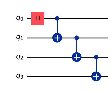
Let’s use a GHZ circuit as the input:
# GHZ Circuit
nq = 4
qc = QuantumCircuit(nq)
qc.h(0)
for i in range(1, nq):
    qc.cx(i-1, i)

qc.draw(output="mpl", style="iqp")

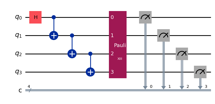
Check that the experiment is appending a random Pauli and measurements as expected:
# Experiment parameters
total_shots = 100000
num_samples = 50
shots = total_shots // num_samples

# Run ideal randomized meas experiment
exp = RandomizedMeasurement(qc, num_samples=num_samples)
exp.circuits()[0].draw(output="mpl", style="iqp")

We now run the experiment with a GHZ circuit on an ideal backend, which produces nearly perfect symmetrical results between \(|0000\rangle\) and \(|1111\rangle\):
expdata_ideal = exp.run(backend_ideal, shots=shots)
counts_ideal = expdata_ideal.analysis_results("counts", dataframe=True).iloc[0].value
print(counts_ideal)
{'1111': 50296, '0000': 49704}
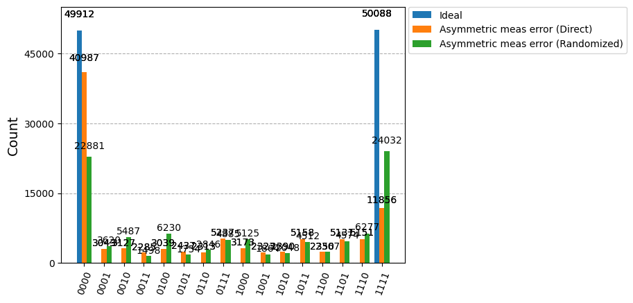
Repeat the experiment on the backend with readout error and compare with results from running GHZ circuit itself:
# Run noisy randomized meas experiment with readout error
expdata_noise = exp.run(noise_backend, shots=shots)
counts_noise = expdata_noise.analysis_results("counts", dataframe=True).iloc[0].value

# Run noisy simulation of the original circuit without randomization
meas_circ = qc.copy()
meas_circ.measure_all()
result = noise_backend.run(meas_circ, shots=total_shots).result()
counts_direct = result.get_counts(0)

from qiskit.visualization import plot_histogram

# Plot counts, ideally randomized one should be more symmetric in noise
# than direct one with asymmetric readout error
plot_histogram([counts_ideal, counts_direct, counts_noise],
            legend=["Ideal",
                    "Asymmetric meas error (Direct)",
                    "Asymmetric meas error (Randomized)"])

For a GHZ state, we expect a symmetric noise model to also produce symmetric readout results. The asymmetric measurement of the original circuit on this backend (Direct on the plot legend) has been successfully symmetrized by the application of randomized measurement (Randomized on the plot legend).
Note that since this experiment tracks the original and added classical registers, it is possible for the original circuit to have its own mid-circuit measurements that would be unaffected by the added randomized measurements, which use its own classical registers:
qc = QuantumCircuit(nq)
qc.h(0)
qc.measure_all()
qc.barrier()
for i in range(1, nq):
    qc.cx(i-1, i)

exp = RandomizedMeasurement(qc, num_samples=num_samples)
exp.circuits()[0].draw(output="mpl", style="iqp")
