Note

This page was generated from docs/tutorials/01_algorithms_introduction.ipynb.

An Introduction to Algorithms using Qiskit

This introduction to algorithms using Qiskit provides a high-level overview to get started with the qiskit_algorithms library.

How is the algorithm library structured?

qiskit_algorithms provides a number of algorithms grouped by category, according to the task they can perform. For instance Minimum Eigensolvers to find the smallest eigen value of an operator, for example ground state energy of a chemistry Hamiltonian or a solution to an optimization problem when expressed as an Ising Hamiltonian. There are Time Evolvers for the time evolution of quantum systems and Amplitude Estimators for value estimation that can be used say in financial applications. The full set of categories can be seen in the documentation link above.

Algorithms are configurable, and part of the configuration will often be in the form of smaller building blocks. For instance VQE, the Variational Quantum Eigensolver, it takes a trial wavefunction, in the form of a QuantumCircuit and a classical optimizer among other things.

Let’s take a look at an example to construct a VQE instance. Here, n_local is the variational form (trial wavefunction), a parameterized circuit which can be varied, and SLSQP a classical optimizer. These are created as separate instances and passed to VQE when it is constructed. Trying, for example, a different classical optimizer, or variational form is simply a case of creating an instance of the one you want and passing it into VQE.

from qiskit_algorithms.optimizers import SLSQP
from qiskit.circuit.library import n_local

num_qubits = 2
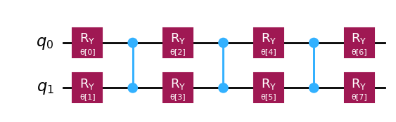
ansatz = n_local(num_qubits, "ry", "cz")
optimizer = SLSQP(maxiter=1000)

Let’s draw the ansatz so we can see it’s a QuantumCircuit where θ[0] through θ[7] will be the parameters that are varied as VQE optimizer finds the minimum eigenvalue. We’ll come back to the parameters later in a working example below.

ansatz.draw("mpl")

But more is needed before we can run the algorithm so let’s get to that next.

How to run an algorithm?

Algorithms rely on the primitives to evaluate expectation values or sample circuits. The primitives can be based on a simulator or real device and can be used interchangeably in the algorithms, as they all implement the same interface.

In the VQE, we have to evaluate expectation values, so for example we can use the qiskit.primitives.StatevectorEstimator which is shipped with the default Qiskit installation.

from qiskit.primitives import StatevectorEstimator

estimator = StatevectorEstimator()

This estimator uses an exact, statevector simulation to evaluate the expectation values. We can also use a noisy simulator or real backends instead. For more information of the simulators you can check out Qiskit Aer and for the actual hardware Qiskit IBM Runtime.

With all the ingredients ready, we can now instantiate the VQE:

from qiskit_algorithms import VQE

vqe = VQE(estimator, ansatz, optimizer)

Now we can call the compute_mininum_eigenvalue() method. The latter is the interface of choice for the application modules, such as Nature and Optimization, in order that they can work interchangeably with any algorithm within the specific category.

A complete working example

Let’s put what we have learned from above together and create a complete working example. VQE will find the minimum eigenvalue, i.e. minimum energy value of a Hamiltonian operator and hence we need such an operator for VQE to work with. Such an operator is given below. This was originally created by the Nature application module as the Hamiltonian for an H2 molecule at 0.735A interatomic distance. It’s a sum of Pauli terms as below.

from qiskit.quantum_info import SparsePauliOp

H2_op = SparsePauliOp.from_list(
    [
        ("II", -1.052373245772859),
        ("IZ", 0.39793742484318045),
        ("ZI", -0.39793742484318045),
        ("ZZ", -0.01128010425623538),
        ("XX", 0.18093119978423156),
    ]
)

So let’s run VQE and print the result object it returns.

result = vqe.compute_minimum_eigenvalue(H2_op)
print(result)

{   'aux_operators_evaluated': None,
    'cost_function_evals': 74,
    'eigenvalue': np.float64(-1.857275026989812),
    'optimal_circuit': <qiskit.circuit.quantumcircuit.QuantumCircuit object at 0x7f9ef4653640>,
    'optimal_parameters': {   ParameterVectorElement(θ[0]): np.float64(1.7487156327559716),
                              ParameterVectorElement(θ[1]): np.float64(4.594349056191267),
                              ParameterVectorElement(θ[2]): np.float64(-5.588483011152245),
                              ParameterVectorElement(θ[3]): np.float64(-2.732337534742184),
                              ParameterVectorElement(θ[4]): np.float64(1.3642962446218774),
                              ParameterVectorElement(θ[5]): np.float64(4.741212465795237),
                              ParameterVectorElement(θ[6]): np.float64(-2.8222154238755026),
                              ParameterVectorElement(θ[7]): np.float64(0.23223071154519628)},
    'optimal_point': array([ 1.74871563,  4.59434906, -5.58848301, -2.73233753,  1.36429624,
        4.74121247, -2.82221542,  0.23223071]),
    'optimal_value': np.float64(-1.857275026989812),
    'optimizer_evals': None,
    'optimizer_result': <qiskit_algorithms.optimizers.optimizer.OptimizerResult object at 0x7f9ea4733340>,
    'optimizer_time': 0.17144560813903809}

From the above result we can see the number of cost function (=energy) evaluations the optimizer took until it found the minimum eigenvalue of \(\approx -1.85727\) which is the electronic ground state energy of the given H2 molecule. The optimal parameters of the ansatz can also be seen which are the values that were in the ansatz at the minimum value.

Updating the primitive inside VQE

Let’s also change the estimator primitive inside the a VQE. Maybe you’re satisfied with the simulation results and now want to use a noisy simulator, or run on hardware!

In this example we’re changing to a noisy estimator, still using Qiskit’s reference primitive. However, you could replace the primitive by e.g. Qiskit Aer’s estimator (qiskit_aer.primitives.EstimatorV2) or even a real backend (qiskit_ibm_runtime.EstimatorV2).

For noisy loss functions, the SPSA optimizer typically performs well, so we also update the optimizer. See also the noisy VQE tutorial for more details on shot-based and noisy simulations.

from qiskit_algorithms.optimizers import SPSA

estimator = StatevectorEstimator(default_precision=1e-2)

vqe.estimator = estimator
vqe.optimizer = SPSA(maxiter=100)
result = vqe.compute_minimum_eigenvalue(operator=H2_op)
print(result)

{   'aux_operators_evaluated': None,
    'cost_function_evals': 200,
    'eigenvalue': np.float64(-1.8538394136177272),
    'optimal_circuit': <qiskit.circuit.quantumcircuit.QuantumCircuit object at 0x7f9ea467ef50>,
    'optimal_parameters': {   ParameterVectorElement(θ[0]): np.float64(-5.845612140276208),
                              ParameterVectorElement(θ[1]): np.float64(3.0801441087482924),
                              ParameterVectorElement(θ[2]): np.float64(0.6724285494011719),
                              ParameterVectorElement(θ[3]): np.float64(-2.2711130325565896),
                              ParameterVectorElement(θ[4]): np.float64(-1.3097422789317397),
                              ParameterVectorElement(θ[5]): np.float64(-0.6405740060047842),
                              ParameterVectorElement(θ[6]): np.float64(4.342132045934191),
                              ParameterVectorElement(θ[7]): np.float64(-6.105095814289072)},
    'optimal_point': array([-5.84561214,  3.08014411,  0.67242855, -2.27111303, -1.30974228,
       -0.64057401,  4.34213205, -6.10509581]),
    'optimal_value': np.float64(-1.8538394136177272),
    'optimizer_evals': None,
    'optimizer_result': <qiskit_algorithms.optimizers.optimizer.OptimizerResult object at 0x7f9ea4733370>,
    'optimizer_time': 0.44191575050354004}

Note: We do not fix the random seed in the simulators here, so re-running gives slightly varying results.

Transpilation options

To close off, if you want to run on real hardware, you’ll be required to transpile your circuits beforehand. In some cases, such as in VQE, the circuit is provided by the user, which means that it can be transpiled beforehand. But in other cases, such as in `Grover <https://qiskit-community.github.io/qiskit-algorithms/stubs/qiskit_algorithms.Grover.html>`__, the class creates its circuit internally.

To deal with this problem, every user-facing class in qiskit-algorithms can be provided with a transpiler and a a transpiler_options keyword-only arguments. The transpiler is any object having a run method that is able to transpile a QuantumCircuit, while the transpiler_options argument is a dictionary of options to be passed to the transpiler’s run method.

As an example, let us define a custom backend on four qubits. Note that this backend has more qubits than our ansatz and our observable.

from qiskit_aer.noise import NoiseModel
from qiskit.providers.fake_provider import GenericBackendV2

coupling_map = [(0, 1), (1, 2), (2, 3)]
backend = GenericBackendV2(num_qubits=4, coupling_map=coupling_map, seed=54)

Let us define a PassManager for this backend.

from qiskit.transpiler.preset_passmanagers import generate_preset_pass_manager

pm = generate_preset_pass_manager(optimization_level=2, backend=backend)

We can then pass this PassManager to the transpiler keyword argument of the VQE constructor. We can also pass any options to the run method of the Transpiler by setting the transpiler_options keyword argument to a dictionary specifying said options. For instance, let us define a callback function that prints out that it has been called on the very first step of the transpilation.

def callback(**kwargs):
    if kwargs["count"] == 0:
        print(f"Callback function has been called!")

We can now build a VQE instance using this PassManager like so.

vqe = VQE(
    estimator, ansatz, SPSA(maxiter=100), transpiler=pm, transpiler_options={"callback": callback}
)
result = vqe.compute_minimum_eigenvalue(operator=H2_op)
print(result)

Callback function has been called!
{   'aux_operators_evaluated': None,
    'cost_function_evals': 200,
    'eigenvalue': np.float64(-1.8569469657029236),
    'optimal_circuit': <qiskit.circuit.quantumcircuit.QuantumCircuit object at 0x7f9ea4622ef0>,
    'optimal_parameters': {   ParameterVectorElement(θ[0]): np.float64(0.6962290518127402),
                              ParameterVectorElement(θ[1]): np.float64(1.0229372106734622),
                              ParameterVectorElement(θ[2]): np.float64(1.0947907620819601),
                              ParameterVectorElement(θ[3]): np.float64(-5.479728800055015),
                              ParameterVectorElement(θ[4]): np.float64(4.601584976727274),
                              ParameterVectorElement(θ[5]): np.float64(-5.379278192725871),
                              ParameterVectorElement(θ[6]): np.float64(1.4358881521598572),
                              ParameterVectorElement(θ[7]): np.float64(4.668146061776705)},
    'optimal_point': array([ 0.69622905,  1.02293721,  1.09479076, -5.4797288 ,  4.60158498,
       -5.37927819,  1.43588815,  4.66814606]),
    'optimal_value': np.float64(-1.8569469657029236),
    'optimizer_evals': None,
    'optimizer_result': <qiskit_algorithms.optimizers.optimizer.OptimizerResult object at 0x7f9ea254fe80>,
    'optimizer_time': 0.9605114459991455}

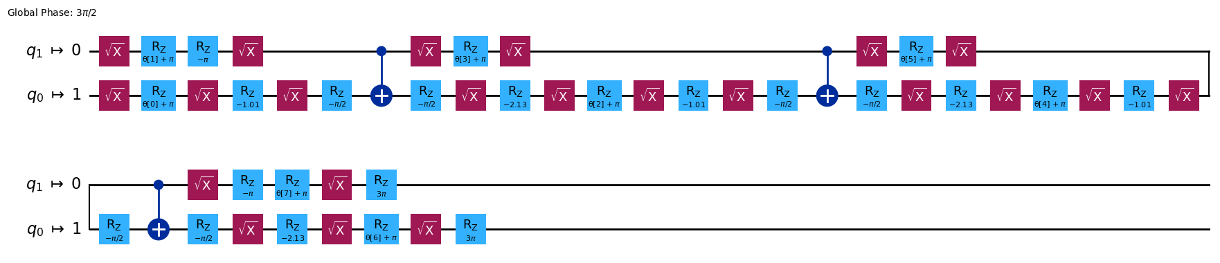
Note that as seen below, the ansatz has automatically been transpiled.

vqe.ansatz.draw("mpl")

This concludes this introduction to algorithms using Qiskit. Please check out the other algorithm tutorials in this series for both broader as well as more in depth coverage of the algorithms.

import tutorial_magics

%qiskit_version_table
%qiskit_copyright

Version Information

Software	Version
qiskit	2.0.3
qiskit_aer	0.17.1
qiskit_algorithms	0.4.0
System information
Python version	3.10.18
OS	Linux
Tue Sep 09 09:43:53 2025 UTC

This code is a part of a Qiskit project

© Copyright IBM 2017, 2025.

This code is licensed under the Apache License, Version 2.0. You may
obtain a copy of this license in the LICENSE.txt file in the root directory
of this source tree or at http://www.apache.org/licenses/LICENSE-2.0.

Any modifications or derivative works of this code must retain this
copyright notice, and modified files need to carry a notice indicating
that they have been altered from the originals.