Note

This page was generated from docs/tutorials/08_cvar_optimization.ipynb.

Improving Variational Quantum Optimization using CVaR

Introduction

This notebook shows how to use the Conditional Value at Risk (CVaR) objective function introduced in [1] within the variational quantum optimization algorithms provided by Qiskit Algorithms. Particularly, it is shown how to setup the MinimumEigenOptimizer using SamplingVQE accordingly. For a given set of shots with corresponding objective values of the considered optimization problem, the CVaR with confidence level \(\alpha \in [0, 1]\) is defined as the average of the \(\alpha\) best shots. Thus, \(\alpha = 1\) corresponds to the standard expected value, while \(\alpha=0\) corresponds to the minimum of the given shots, and \(\alpha \in (0, 1)\) is a tradeoff between focusing on better shots, but still applying some averaging to smoothen the optimization landscape.

References

[1] P. Barkoutsos et al., Improving Variational Quantum Optimization using CVaR, Quantum 4, 256 (2020).

import matplotlib.pyplot as plt
import numpy as np
from docplex.mp.model import Model
from qiskit.circuit.library import real_amplitudes
from qiskit.primitives import StatevectorSampler
from qiskit_optimization.algorithms import MinimumEigenOptimizer
from qiskit_optimization.converters import LinearEqualityToPenalty
from qiskit_optimization.minimum_eigensolvers import NumPyMinimumEigensolver, SamplingVQE
from qiskit_optimization.optimizers import COBYLA
from qiskit_optimization.translators import from_docplex_mp
from qiskit_optimization.utils import algorithm_globals

/tmp/ipykernel_16022/311796302.py:4: DeprecationWarning: Using Qiskit with Python 3.9 is deprecated as of the 2.1.0 release. Support for running Qiskit with Python 3.9 will be removed in the 2.3.0 release, which coincides with when Python 3.9 goes end of life.
  from qiskit.circuit.library import real_amplitudes

algorithm_globals.random_seed = 123456

Portfolio Optimization

In the following we define a problem instance for portfolio optimization as introduced in [1].

# prepare problem instance
n = 6  # number of assets
q = 0.5  # risk factor
budget = n // 2  # budget
penalty = 2 * n  # scaling of penalty term

# instance from [1]
mu = np.array([0.7313, 0.9893, 0.2725, 0.8750, 0.7667, 0.3622])
sigma = np.array(
    [
        [0.7312, -0.6233, 0.4689, -0.5452, -0.0082, -0.3809],
        [-0.6233, 2.4732, -0.7538, 2.4659, -0.0733, 0.8945],
        [0.4689, -0.7538, 1.1543, -1.4095, 0.0007, -0.4301],
        [-0.5452, 2.4659, -1.4095, 3.5067, 0.2012, 1.0922],
        [-0.0082, -0.0733, 0.0007, 0.2012, 0.6231, 0.1509],
        [-0.3809, 0.8945, -0.4301, 1.0922, 0.1509, 0.8992],
    ]
)

# or create random instance
# mu, sigma = portfolio.random_model(n, seed=123)  # expected returns and covariance matrix

# create docplex model
mdl = Model("portfolio_optimization")
x = mdl.binary_var_list(range(n), name="x")
objective = mdl.sum([mu[i] * x[i] for i in range(n)])
objective -= q * mdl.sum([sigma[i, j] * x[i] * x[j] for i in range(n) for j in range(n)])
mdl.maximize(objective)
mdl.add_constraint(mdl.sum(x[i] for i in range(n)) == budget)

# case to
qp = from_docplex_mp(mdl)

# solve classically as reference
opt_result = MinimumEigenOptimizer(NumPyMinimumEigensolver()).solve(qp)
print(opt_result.prettyprint())

objective function value: 1.27835
variable values: x_0=1.0, x_1=1.0, x_2=0.0, x_3=0.0, x_4=1.0, x_5=0.0
status: SUCCESS

# we convert the problem to an unconstrained problem for further analysis,
# otherwise this would not be necessary as the MinimumEigenSolver would do this
# translation automatically
linear2penalty = LinearEqualityToPenalty(penalty=penalty)
qp = linear2penalty.convert(qp)
_, offset = qp.to_ising()

Minimum Eigen Optimizer using SamplingVQE

# set classical optimizer
maxiter = 100
optimizer = COBYLA(maxiter=maxiter)

# set variational ansatz
ansatz = real_amplitudes(n, reps=1)
m = ansatz.num_parameters

# set sampler
sampler = StatevectorSampler(seed=123, default_shots=1000)

# run variational optimization for different values of alpha
alphas = [1.0, 0.50, 0.25]  # confidence levels to be evaluated

# dictionaries to store optimization progress and results
objectives = {alpha: [] for alpha in alphas}  # set of tested objective functions w.r.t. alpha
results = {}  # results of minimum eigensolver w.r.t alpha


# callback to store intermediate results
def callback(i, params, obj, stddev, alpha):
    # we translate the objective from the internal Ising representation
    # to the original optimization problem
    objectives[alpha].append(np.real_if_close(-(obj + offset)))


# loop over all given alpha values
for alpha in alphas:

    # initialize SamplingVQE using CVaR
    vqe = SamplingVQE(
        sampler=sampler,
        ansatz=ansatz,
        optimizer=optimizer,
        aggregation=alpha,
        callback=lambda i, params, obj, stddev: callback(i, params, obj, stddev, alpha),
    )

    # initialize optimization algorithm based on CVaR-SamplingVQE
    opt_alg = MinimumEigenOptimizer(vqe)

    # solve problem
    results[alpha] = opt_alg.solve(qp)

    # print results
    print("alpha = {}:".format(alpha))
    print(results[alpha].prettyprint())
    print()

alpha = 1.0:
objective function value: 0.7296000000000049
variable values: x_0=0.0, x_1=1.0, x_2=1.0, x_3=0.0, x_4=1.0, x_5=0.0
status: SUCCESS

alpha = 0.5:
objective function value: 1.2783500000000174
variable values: x_0=1.0, x_1=1.0, x_2=0.0, x_3=0.0, x_4=1.0, x_5=0.0
status: SUCCESS

alpha = 0.25:
objective function value: 1.2783500000000174
variable values: x_0=1.0, x_1=1.0, x_2=0.0, x_3=0.0, x_4=1.0, x_5=0.0
status: SUCCESS

# plot resulting history of objective values
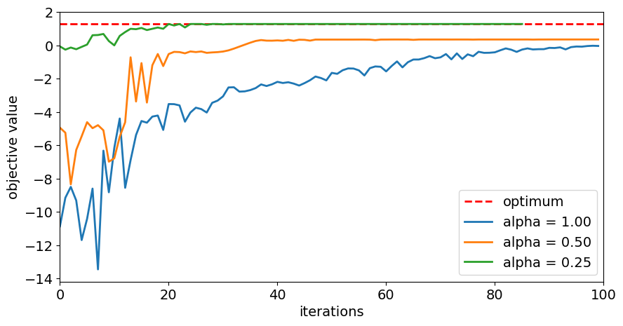
plt.figure(figsize=(10, 5))
plt.plot([0, maxiter], [opt_result.fval, opt_result.fval], "r--", linewidth=2, label="optimum")
for alpha in alphas:
    plt.plot(objectives[alpha], label="alpha = %.2f" % alpha, linewidth=2)
plt.legend(loc="lower right", fontsize=14)
plt.xlim(0, maxiter)
plt.xticks(fontsize=14)
plt.xlabel("iterations", fontsize=14)
plt.yticks(fontsize=14)
plt.ylabel("objective value", fontsize=14)
plt.show()

# evaluate and sort all objective values
objective_values = np.zeros(2**n)
for i in range(2**n):
    x_bin = ("{0:0%sb}" % n).format(i)
    x = [0 if x_ == "0" else 1 for x_ in reversed(x_bin)]
    objective_values[i] = qp.objective.evaluate(x)
ind = np.argmax(objective_values)

# evaluate final optimal probability for each alpha
for alpha in alphas:
    probabilities = np.zeros(2**n)
    prob_dict = results[alpha].min_eigen_solver_result.eigenstate.binary_probabilities()
    for key, val in prob_dict.items():
        probabilities[int(key, 2)] = val
    print("optimal probability (alpha = %.2f):  %.4f" % (alpha, probabilities[ind]))

optimal probability (alpha = 1.00):  0.0000
optimal probability (alpha = 0.50):  0.0050
optimal probability (alpha = 0.25):  0.3010

import tutorial_magics

%qiskit_version_table
%qiskit_copyright

Version Information

Software	Version
qiskit	2.1.2
qiskit_optimization	0.7.0
System information
Python version	3.9.23
OS	Linux
Wed Aug 20 14:17:30 2025 UTC

This code is a part of a Qiskit project

© Copyright IBM 2017, 2025.

This code is licensed under the Apache License, Version 2.0. You may
obtain a copy of this license in the LICENSE.txt file in the root directory
of this source tree or at http://www.apache.org/licenses/LICENSE-2.0.

Any modifications or derivative works of this code must retain this
copyright notice, and modified files need to carry a notice indicating
that they have been altered from the originals.