Note
இந்தப் பக்கம் docs/tutorials/02_neural_network_classifier_and_regressor.ipynb இலிருந்து உருவாக்கப்பட்டது.
நரம்பியல் நெட்வொர்க் வகைப்படுத்தி & பின்னடைவு#
இந்த டுடோரியலில் NeuralNetworkClassifier மற்றும் NeuralNetworkRegressor எவ்வாறு பயன்படுத்தப்படுகின்றன என்பதைக் காட்டுகிறோம். இருவரும் ஒரு உள்ளீடாக ஒரு (குவாண்டம்) NeuralNetwork ஐ எடுத்து ஒரு குறிப்பிட்ட சூழலில் பயன்படுத்துகிறார்கள். இரண்டு நிகழ்வுகளிலும் வசதிக்காக முன்பே உள்ளமைக்கப்பட்ட மாறுபாட்டை நாங்கள் வழங்குகிறோம், மாறுபட்ட குவாண்டம் வகைப்படுத்தி (VQC) மற்றும் மாறுபட்ட குவாண்டம் பின்னடைவு (VQR). பயிற்சி பின்வருமாறு கட்டமைக்கப்பட்டுள்ளது:
Classification
EstimatorQNNஉடன் வகைப்படுத்துதல்SamplerQNNஉடன் வகைப்படுத்துதல்மாறுபட்ட குவாண்டம் வகைப்படுத்தி (
VQC)
Regression
EstimatorQNNஉடன் பின்னடைவுமாறுபட்ட குவாண்டம் பின்னடைவு (`` VQR``)
[1]:
import matplotlib.pyplot as plt
import numpy as np
from IPython.display import clear_output
from qiskit import QuantumCircuit
from qiskit.circuit import Parameter
from qiskit.circuit.library import RealAmplitudes, ZZFeatureMap
from qiskit_algorithms.optimizers import COBYLA, L_BFGS_B
from qiskit_algorithms.utils import algorithm_globals

from qiskit_machine_learning.algorithms.classifiers import NeuralNetworkClassifier, VQC
from qiskit_machine_learning.algorithms.regressors import NeuralNetworkRegressor, VQR
from qiskit_machine_learning.neural_networks import SamplerQNN, EstimatorQNN
from qiskit_machine_learning.circuit.library import QNNCircuit

algorithm_globals.random_seed = 42
வகைப்படுத்துதல்#
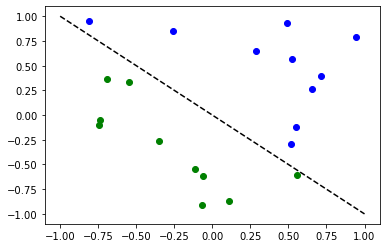
பின்வரும் வழிமுறைகளை விளக்குவதற்கு எளிய வகைப்பாடு தரவுத்தொகுப்பை நாங்கள் தயார் செய்கிறோம்.
[2]:
num_inputs = 2
num_samples = 20
X = 2 * algorithm_globals.random.random([num_samples, num_inputs]) - 1
y01 = 1 * (np.sum(X, axis=1) >= 0)  # in { 0,  1}
y = 2 * y01 - 1  # in {-1, +1}
y_one_hot = np.zeros((num_samples, 2))
for i in range(num_samples):
    y_one_hot[i, y01[i]] = 1

for x, y_target in zip(X, y):
    if y_target == 1:
        plt.plot(x[0], x[1], "bo")
    else:
        plt.plot(x[0], x[1], "go")
plt.plot([-1, 1], [1, -1], "--", color="black")
plt.show()
EstimatorQNN உடன் வகைப்படுத்துதல்#
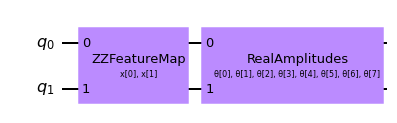
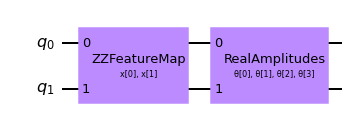
First we show how an EstimatorQNN can be used for classification within a NeuralNetworkClassifier. In this context, the EstimatorQNN is expected to return one-dimensional output in \([-1, +1]\). This only works for binary classification and we assign the two classes to \(\{-1, +1\}\). To simplify the composition of parameterized quantum circuit from a feature map and an ansatz we can use the QNNCircuit class.
[3]:
# construct QNN with the QNNCircuit's default ZZFeatureMap feature map and RealAmplitudes ansatz.
qc = QNNCircuit(num_qubits=2)
qc.draw(output="mpl")
[3]:
ஒரு குவாண்டம் நியூரல் நெட்வொர்க்கை உருவாக்கவும்
[4]:
estimator_qnn = EstimatorQNN(circuit=qc)
[5]:
# QNN maps inputs to [-1, +1]
estimator_qnn.forward(X[0, :], algorithm_globals.random.random(estimator_qnn.num_weights))
[5]:
array([[0.23521988]])
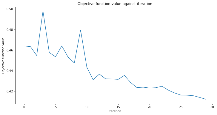
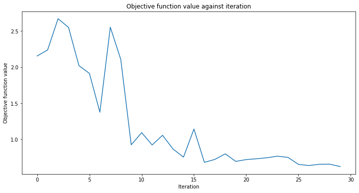
callback_graph எனப்படும் திரும்ப அழைக்கும் செயல்பாட்டைச் சேர்ப்போம். இது ஆப்டிமைசரின் ஒவ்வொரு மறு செய்கைக்கும் அழைக்கப்படும் மற்றும் இரண்டு அளவுருக்கள் அனுப்பப்படும்: தற்போதைய எடைகள் மற்றும் அந்த எடைகளில் புறநிலை செயல்பாட்டின் மதிப்பு. எங்கள் செயல்பாட்டிற்காக, புறநிலை செயல்பாட்டின் மதிப்பை ஒரு வரிசையில் சேர்க்கிறோம், எனவே மறு செய்கை மற்றும் புறநிலை செயல்பாட்டு மதிப்புக்கு எதிராக திட்டமிடலாம் மற்றும் ஒவ்வொரு மறு செய்கையுடன் வரைபடத்தைப் புதுப்பிக்கலாம். இருப்பினும், குறிப்பிடப்பட்ட இரண்டு அளவுருக்களைப் பெறும் வரை நீங்கள் திரும்ப அழைக்கும் செயல்பாட்டின் மூலம் நீங்கள் விரும்பியதைச் செய்யலாம்.
[6]:
# callback function that draws a live plot when the .fit() method is called
def callback_graph(weights, obj_func_eval):
    clear_output(wait=True)
    objective_func_vals.append(obj_func_eval)
    plt.title("Objective function value against iteration")
    plt.xlabel("Iteration")
    plt.ylabel("Objective function value")
    plt.plot(range(len(objective_func_vals)), objective_func_vals)
    plt.show()
[7]:
# construct neural network classifier
estimator_classifier = NeuralNetworkClassifier(
    estimator_qnn, optimizer=COBYLA(maxiter=60), callback=callback_graph
)
[8]:
# create empty array for callback to store evaluations of the objective function
objective_func_vals = []
plt.rcParams["figure.figsize"] = (12, 6)

# fit classifier to data
estimator_classifier.fit(X, y)

# return to default figsize
plt.rcParams["figure.figsize"] = (6, 4)

# score classifier
estimator_classifier.score(X, y)
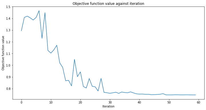
[8]:
0.8
[9]:
# evaluate data points
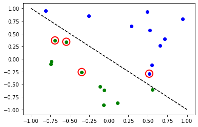
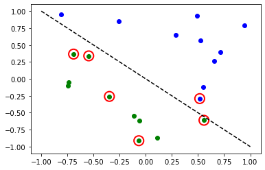
y_predict = estimator_classifier.predict(X)
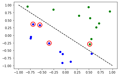
# plot results
# red == wrongly classified
for x, y_target, y_p in zip(X, y, y_predict):
if y_target == 1:
plt.plot(x[0], x[1], "bo")
else:
plt.plot(x[0], x[1], "go")
if y_target != y_p:
plt.scatter(x[0], x[1], s=200, facecolors="none", edgecolors="r", linewidths=2)
plt.plot([-1, 1], [1, -1], "--", color="black")
plt.show()
இப்போது, மாதிரி பயிற்சியளிக்கப்படும்போது, நரம்பியல் வலையமைப்பின் எடைகளை நாம் ஆராயலாம். தயவுசெய்து கவனிக்கவும், எடைகளின் எண்ணிக்கை ansatz மூலம் வரையறுக்கப்படுகிறது.
[10]:
estimator_classifier.weights
[10]:
array([ 7.99142399e-01, -1.02869770e+00, -1.32131512e-04, -3.47046684e-01,
        1.13636802e+00,  6.56831727e-01,  2.17902158e+00, -1.08678332e+00])
SamplerQNN உடன் வகைப்படுத்துதல்#
Next we show how a SamplerQNN can be used for classification within a NeuralNetworkClassifier. In this context, the SamplerQNN is expected to return \(d\)-dimensional probability vector as output, where \(d\) denotes the number of classes. The underlying Sampler primitive returns quasi-distributions of bit strings and we just need to define a mapping from the measured bitstrings to the different classes. For binary classification we use the parity mapping. Again we can
use the QNNCircuit class to set up a parameterized quantum circuit from a feature map and ansatz of our choice.
[11]:
# construct a quantum circuit from the default ZZFeatureMap feature map and a customized RealAmplitudes ansatz
qc = QNNCircuit(ansatz=RealAmplitudes(num_inputs, reps=1))
qc.draw(output="mpl")
[11]:
[12]:
# parity maps bitstrings to 0 or 1
def parity(x):
    return "{:b}".format(x).count("1") % 2


output_shape = 2  # corresponds to the number of classes, possible outcomes of the (parity) mapping.
[13]:
# construct QNN
sampler_qnn = SamplerQNN(
    circuit=qc,
    interpret=parity,
    output_shape=output_shape,
)
[14]:
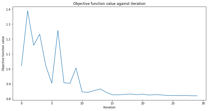
# construct classifier
sampler_classifier = NeuralNetworkClassifier(
    neural_network=sampler_qnn, optimizer=COBYLA(maxiter=30), callback=callback_graph
)
[15]:
# create empty array for callback to store evaluations of the objective function
objective_func_vals = []
plt.rcParams["figure.figsize"] = (12, 6)

# fit classifier to data
sampler_classifier.fit(X, y01)

# return to default figsize
plt.rcParams["figure.figsize"] = (6, 4)

# score classifier
sampler_classifier.score(X, y01)
[15]:
0.7
[16]:
# evaluate data points
y_predict = sampler_classifier.predict(X)

# plot results
# red == wrongly classified
for x, y_target, y_p in zip(X, y01, y_predict):
    if y_target == 1:
        plt.plot(x[0], x[1], "bo")
    else:
        plt.plot(x[0], x[1], "go")
    if y_target != y_p:
        plt.scatter(x[0], x[1], s=200, facecolors="none", edgecolors="r", linewidths=2)
plt.plot([-1, 1], [1, -1], "--", color="black")
plt.show()
மீண்டும், மாதிரிப் பயிற்சி பெற்றவுடன் நாம் எடைகளைப் பார்க்கலாம். எங்கள் ansatz இல் வெளிப்படையாக reps=1 அமைக்கும்போது, முந்தைய மாதிரியைவிட குறைவான அளவுருக்களைக் காணலாம்.
[17]:
sampler_classifier.weights
[17]:
array([ 1.67198565, 0.46045402, -0.93462862, -0.95266092])
மாறுபட்ட குவாண்டம் வகைப்படுத்தி (VQC)#
VQC என்பது SamplerQNN உடன் NeuralNetworkClassifier``ன் ஒரு சிறப்பு மாறுபாடு ஆகும். இது பிட்ஸ்ட்ரிங்கில் இருந்து வகைப்பாடு வரை வரைபடத்திற்கு ஒரு சமநிலை மேப்பிங்கை (அல்லது பல வகுப்புகளுக்கு நீட்டிப்புகள்) பயன்படுத்துகிறது, இதன் விளைவாக ஒரு நிகழ்தகவு திசையன் ஏற்படுகிறது, இது ஒரு சூடான குறியிடப்பட்ட முடிவாக விளக்கப்படுகிறது. இயல்பாக, இது ஒரு சூடான குறியாக்கப்பட்ட வடிவத்தில் கொடுக்கப்பட்ட லேபிள்களை எதிர்பார்க்கும் ``CrossEntropyLoss செயல்பாட்டைப் பயன்படுத்துகிறது மற்றும் அந்த வடிவமைப்பிலும் கணிப்புகளை வழங்கும்.
[18]:
# construct feature map, ansatz, and optimizer
feature_map = ZZFeatureMap(num_inputs)
ansatz = RealAmplitudes(num_inputs, reps=1)

# construct variational quantum classifier
vqc = VQC(
    feature_map=feature_map,
    ansatz=ansatz,
    loss="cross_entropy",
    optimizer=COBYLA(maxiter=30),
    callback=callback_graph,
)
[19]:
# create empty array for callback to store evaluations of the objective function
objective_func_vals = []
plt.rcParams["figure.figsize"] = (12, 6)

# fit classifier to data
vqc.fit(X, y_one_hot)

# return to default figsize
plt.rcParams["figure.figsize"] = (6, 4)

# score classifier
vqc.score(X, y_one_hot)
[19]:
0.8
[20]:
# evaluate data points
y_predict = vqc.predict(X)

# plot results
# red == wrongly classified
for x, y_target, y_p in zip(X, y_one_hot, y_predict):
    if y_target[0] == 1:
        plt.plot(x[0], x[1], "bo")
    else:
        plt.plot(x[0], x[1], "go")
    if not np.all(y_target == y_p):
        plt.scatter(x[0], x[1], s=200, facecolors="none", edgecolors="r", linewidths=2)
plt.plot([-1, 1], [1, -1], "--", color="black")
plt.show()
VQC உடன் பல வகுப்புகள்#
இந்தப் பிரிவில், மூன்று வகுப்புகளின் மாதிரிகளைக் கொண்ட செயற்கைத் தரவுத்தொகுப்பை உருவாக்கி, இந்தத் தரவுத்தொகுப்பை வகைப்படுத்துவதற்கு ஒரு மாதிரியைப் பயிற்றுவிப்பது எப்படி என்பதைக் காட்டுகிறோம். இயந்திர கற்றலில் மிகவும் சுவாரஸ்யமான சிக்கல்களை எவ்வாறு சமாளிப்பது என்பதை இந்த எடுத்துக்காட்டு காட்டுகிறது. நிச்சயமாக, குறுகிய பயிற்சி நேரத்திற்காக நாங்கள் ஒரு சிறிய தரவுத்தொகுப்பை தயார் செய்கிறோம். தரவுத்தொகுப்பை உருவாக்க SciKit-Learn இலிருந்து make_classification ஐப் பயன்படுத்துகிறோம். தரவுத்தொகுப்பில் 10 மாதிரிகள் உள்ளன, 2 அம்சங்கள், அதாவது தரவுத்தொகுப்பின் நல்ல சதித்திட்டத்தை நாம் இன்னும் வைத்திருக்க முடியும், அதே போல் தேவையற்ற அம்சங்கள் எதுவும் இல்லை, இவை மற்ற அம்சங்களின் கலவையாக உருவாக்கப்பட்ட அம்சங்கள். மேலும், தரவுத்தொகுப்பில் எங்களிடம் 3 வெவ்வேறு வகுப்புகள் உள்ளன, ஒவ்வொரு வகுப்புகளும் ஒரு வகையான சென்ட்ராய்டு மற்றும் வகுப்பைப் பிரிப்பதை 2.0 ஆக அமைக்கிறோம், வகைப்படுத்தல் சிக்கலை எளிதாக்க, இயல்புநிலை மதிப்பான 1.0 இலிருந்து சிறிது அதிகரிப்பு.
தரவுத்தொகுப்பு உருவாக்கப்பட்டவுடன் அம்சங்களை [0, 1] வரம்பிற்குள் அளவிடுவோம்.
[21]:
from sklearn.datasets import make_classification
from sklearn.preprocessing import MinMaxScaler

X, y = make_classification(
    n_samples=10,
    n_features=2,
    n_classes=3,
    n_redundant=0,
    n_clusters_per_class=1,
    class_sep=2.0,
    random_state=algorithm_globals.random_seed,
)
X = MinMaxScaler().fit_transform(X)
நமது தரவுத்தொகுப்பு எப்படி இருக்கிறது என்று பார்ப்போம்.
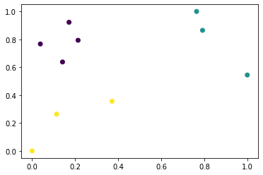
[22]:
plt.scatter(X[:, 0], X[:, 1], c=y)
[22]:
<matplotlib.collections.PathCollection at 0x7fd5e072c250>
நாங்கள் லேபிள்களை மாற்றி அவற்றை வகைப்படுத்துகிறோம்.
[23]:
y_cat = np.empty(y.shape, dtype=str)
y_cat[y == 0] = "A"
y_cat[y == 1] = "B"
y_cat[y == 2] = "C"
print(y_cat)
['A' 'A' 'B' 'C' 'C' 'A' 'B' 'B' 'A' 'C']
முந்தைய உதாரணத்தைப் போலவே VQC இன் நிகழ்வை உருவாக்குகிறோம், ஆனால் இந்த விஷயத்தில் நாம் குறைந்தபட்ச அளவுருக்களை அனுப்புகிறோம். அம்ச வரைபடம் மற்றும் அன்சாட்ஸுக்குப் பதிலாக, தரவுத்தொகுப்பில் உள்ள அம்சங்களின் எண்ணிக்கைக்கு சமமான குவிட்களின் எண்ணிக்கையை மட்டுமே கடந்து செல்கிறோம், பயிற்சி நேரத்தைக் குறைக்க குறைந்த எண்ணிக்கையிலான மறு செய்கையுடன் கூடிய ஆப்டிமைசர், ஒரு குவாண்டம் நிகழ்வு மற்றும் முன்னேற்றத்தைக் காண திரும்பவும்.
[24]:
vqc = VQC(
    num_qubits=2,
    optimizer=COBYLA(maxiter=30),
    callback=callback_graph,
)
முந்தைய எடுத்துக்காட்டுகளைப் போலவே பயிற்சி செயல்முறையைத் தொடங்கவும்.
[25]:
# create empty array for callback to store evaluations of the objective function
objective_func_vals = []
plt.rcParams["figure.figsize"] = (12, 6)

# fit classifier to data
vqc.fit(X, y_cat)

# return to default figsize
plt.rcParams["figure.figsize"] = (6, 4)

# score classifier
vqc.score(X, y_cat)
[25]:
0.9
எங்களிடம் குறைந்த எண்ணிக்கையிலான மறு செய்கைகள் இருந்தபோதிலும், நாங்கள் நல்ல மதிப்பெண்ணைப் பெற்றுள்ளோம். முன்கணிப்பு முறையின் வெளியீட்டைப் பார்க்கலாம் மற்றும் வெளியீட்டை அடிப்படை உண்மையுடன் ஒப்பிடலாம்.
[26]:
predict = vqc.predict(X)
print(f"Predicted labels: {predict}")
print(f"Ground truth:     {y_cat}")
Predicted labels: ['A' 'A' 'B' 'C' 'C' 'A' 'B' 'B' 'A' 'B']
Ground truth:     ['A' 'A' 'B' 'C' 'C' 'A' 'B' 'B' 'A' 'C']
பின்னடைவு#
பின்வரும் வழிமுறைகளை விளக்குவதற்கு எளிய பின்னடைவு தரவுத்தொகுப்பை நாங்கள் தயார் செய்கிறோம்.
[27]:
num_samples = 20
eps = 0.2
lb, ub = -np.pi, np.pi
X_ = np.linspace(lb, ub, num=50).reshape(50, 1)
f = lambda x: np.sin(x)

X = (ub - lb) * algorithm_globals.random.random([num_samples, 1]) + lb
y = f(X[:, 0]) + eps * (2 * algorithm_globals.random.random(num_samples) - 1)

plt.plot(X_, f(X_), "r--")
plt.plot(X, y, "bo")
plt.show()
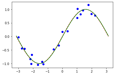
EstimatorQNN உடன் பின்னடைவு#
இங்கு மதிப்புகளை \([-1, +1]\) இல் வழங்கும் EstimatorQNN மூலம் பின்னடைவைக் கட்டுப்படுத்துகிறோம். மிகவும் சிக்கலான மற்றும் பல பரிமாண மாதிரிகள் உருவாக்கப்படலாம், மேலும் SamplerQNN அடிப்படையிலும் உருவாக்கப்படலாம் ஆனால் அது இந்த டுடோரியலின் நோக்கத்தை மீறுகிறது.
[28]:
# construct simple feature map
param_x = Parameter("x")
feature_map = QuantumCircuit(1, name="fm")
feature_map.ry(param_x, 0)

# construct simple ansatz
param_y = Parameter("y")
ansatz = QuantumCircuit(1, name="vf")
ansatz.ry(param_y, 0)

# construct a circuit
qc = QNNCircuit(feature_map=feature_map, ansatz=ansatz)

# construct QNN
regression_estimator_qnn = EstimatorQNN(circuit=qc)
[29]:
# construct the regressor from the neural network
regressor = NeuralNetworkRegressor(
    neural_network=regression_estimator_qnn,
    loss="squared_error",
    optimizer=L_BFGS_B(maxiter=5),
    callback=callback_graph,
)
[30]:
# create empty array for callback to store evaluations of the objective function
objective_func_vals = []
plt.rcParams["figure.figsize"] = (12, 6)

# fit to data
regressor.fit(X, y)

# return to default figsize
plt.rcParams["figure.figsize"] = (6, 4)

# score the result
regressor.score(X, y)
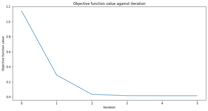
[30]:
0.9769994291935522
[31]:
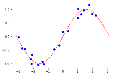
# plot target function
plt.plot(X_, f(X_), "r--")

# plot data
plt.plot(X, y, "bo")

# plot fitted line
y_ = regressor.predict(X_)
plt.plot(X_, y_, "g-")
plt.show()
வகைப்பாடு மாதிரிகளைப் போலவே, மாதிரியின் தொடர்புடைய பண்புகளை வினவுவதன் மூலம் பயிற்சி பெற்ற எடைகளின் வரிசையைப் பெறலாம். இந்த மாதிரியில் மேலே param_y என வரையறுக்கப்பட்ட ஒரு அளவுரு மட்டுமே உள்ளது.
[32]:
regressor.weights
[32]:
array([-1.58870599])
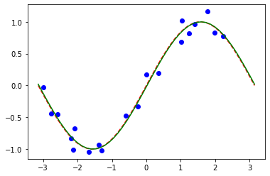
மாறுபட்ட குவாண்டம் பின்னடைவுடன் பின்னடைவு (VQR)#
வகைப்படுத்தலுக்கான VQC` போன்றது, ``VQR` என்பது ``EstimatorQNN உடன் NeuralNetworkRegressor``ன் சிறப்பு மாறுபாடாகும். முன்னறிவிப்புகள் மற்றும் இலக்குகளுக்கு இடையே சராசரி ஸ்கொயர் பிழையைக் குறைக்க, இயல்பாக இது ``L2Loss செயல்பாட்டைக் கருதுகிறது.
[33]:
vqr = VQR(
    feature_map=feature_map,
    ansatz=ansatz,
    optimizer=L_BFGS_B(maxiter=5),
    callback=callback_graph,
)
[34]:
# create empty array for callback to store evaluations of the objective function
objective_func_vals = []
plt.rcParams["figure.figsize"] = (12, 6)

# fit regressor
vqr.fit(X, y)

# return to default figsize
plt.rcParams["figure.figsize"] = (6, 4)

# score result
vqr.score(X, y)
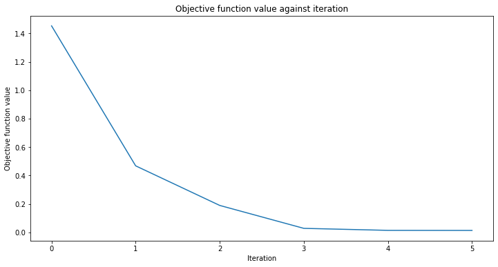
[34]:
0.9769955693935385
[35]:
# plot target function
plt.plot(X_, f(X_), "r--")

# plot data
plt.plot(X, y, "bo")

# plot fitted line
y_ = vqr.predict(X_)
plt.plot(X_, y_, "g-")
plt.show()
[36]:
import qiskit.tools.jupyter

%qiskit_version_table
%qiskit_copyright
Version Information
| Qiskit Software | Version |
|---|---|
qiskit-terra | 0.24.0 |
qiskit-aer | 0.12.0 |
qiskit-ignis | 0.6.0 |
qiskit-ibmq-provider | 0.20.2 |
qiskit | 0.43.0 |
qiskit-machine-learning | 0.7.0 |
| System information | |
| Python version | 3.8.8 |
| Python compiler | Clang 10.0.0 |
| Python build | default, Apr 13 2021 12:59:45 |
| OS | Darwin |
| CPUs | 8 |
| Memory (Gb) | 32.0 |
| Tue Jun 13 16:39:30 2023 CEST | |
This code is a part of Qiskit
© Copyright IBM 2017, 2023.
This code is licensed under the Apache License, Version 2.0. You may
obtain a copy of this license in the LICENSE.txt file in the root directory
of this source tree or at http://www.apache.org/licenses/LICENSE-2.0.
Any modifications or derivative works of this code must retain this
copyright notice, and modified files need to carry a notice indicating
that they have been altered from the originals.