Building and solving models of quantum systems¶

In this tutorial we will walk through the simulation of a two-transmon system using the high level systems modelling module.

We will proceed in the following steps:

Define the model for the system as the summation of two transmon models with an exchange interaction.
Construct a DressedBasis object storing the dressed basis for the model.
Simulate the time evolution under driving of one of the transmons, starting in the ground state.
Restrict the DressedBasis to the computational subspace, and plot the populations of the computational states as a function of time under the above time evolution.

First, we set JAX to work in 64 bit mode on CPU.

import jax
jax.config.update("jax_enable_x64", True)

# tell JAX we are using CPU
jax.config.update('jax_platform_name', 'cpu')

1. Define the two transmon model¶

First, define a single transmon, modelled as a Duffing oscillator. We will use a 3-dimensional model.

from qiskit_dynamics.systems import Subsystem, DuffingOscillator

# subsystem the model is to be defined on
Q0 = Subsystem("0", dim=3)

# the model
Q0_model = DuffingOscillator(
    subsystem=Q0,
    frequency=5.,
    anharm=-0.33,
    drive_strength=0.01
)

Print the model to see its contents.

print(str(Q0_model))

QuantumSystemModel(
    static_hamiltonian=31.41592653589793 * N(0) + (-1.0367255756846319 * N(0) @ (N(0) + -1 * I(0))),
    drive_hamiltonian_coefficients=['d0'],
    drive_hamiltonians=[0.06283185307179587 * X(0)],
    static_dissipators=[],
    drive_dissipator_coefficients=[],
    drive_dissipators=[],
)

Define a model for the second transmon, an exchange interaction, and add the models together.

from qiskit_dynamics.systems import ExchangeInteraction

# subsytem for second transmon
Q1 = Subsystem("1", 3)

# model for second transmon
Q1_model = DuffingOscillator(
    subsystem=Q1,
    frequency=5.05,
    anharm=-0.33,
    drive_strength=0.01
)

# model for coupling
coupling_model = ExchangeInteraction(
    subsystems=[Q0, Q1],
    g=0.002
)

two_transmon_model = Q0_model + Q1_model + coupling_model

Printing the string representation of the full two_transmon_model shows how the different components are combined by model addition.

print(str(two_transmon_model))

QuantumSystemModel(
    static_hamiltonian=((31.41592653589793 * N(0) + (-1.0367255756846319 * N(0) @ (N(0) + -1 * I(0)))) + (31.73008580125691 * N(1) + (-1.0367255756846319 * N(1) @ (N(1) + -1 * I(1))))) + 0.012566370614359173 * X(0) @ X(1),
    drive_hamiltonian_coefficients=['d0', 'd1'],
    drive_hamiltonians=[0.06283185307179587 * X(0), 0.06283185307179587 * X(1)],
    static_dissipators=[],
    drive_dissipator_coefficients=[],
    drive_dissipators=[],
)

2. Construct the dressed basis¶

The initial state and results will be computed in terms of the dressed basis. Call the dressed_basis method of the model to construct the DressedBasis instance corresponding to this model.

dressed_basis = two_transmon_model.dressed_basis()

3. Simulate the evolution of the system under a constant drive envelope on one of the transmons¶

Using the solve method, run a simulation under a constant drive envelope on transmon 0. Note that in contrast to previous interfaces, like the Solver class, the signals are passed as a dictionary mapping coefficient names to the Signal instance.

Use the ground state as the initial state, accessible via the ground_state property of the DressedBasis object.

import numpy as np
from qiskit_dynamics import Signal

tf = 0.5 / 0.01
t_span = np.array([0., tf])
t_eval = np.linspace(0., t_span[-1], 50)

result = two_transmon_model.solve(
    signals={"d0": Signal(1., carrier_freq=5.)},
    t_span=t_span,
    t_eval=t_eval,
    y0=dressed_basis.ground_state,
    atol=1e-10,
    rtol=1e-10,
    method="jax_odeint"
)

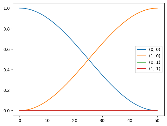
4. Plot the populations of the computational states during the above time evolution¶

First, we restrict the dressed basis to only the computational states, via the computational_states property.

computational_states = dressed_basis.computational_states

The populations of observing a given state in one of the computational states can be computed via the ONBasis.probabilities() method. For example, we can compute them for the final state:

probabilities = computational_states.probabilities(result.y[-1])
for label, probability in zip(computational_states.labels, probabilities):
    print(f'{label["index"]}: {probability}')

(0, 0): 4.004997730961459e-05
(1, 0): 0.9995300652773764
(0, 1): 2.1738884619151254e-09
(1, 1): 1.0406941537117426e-06

Applying this function to every intermediate time point, generate a plot of the computational state populations over the full time evolution:

import matplotlib.pyplot as plt
from jax import vmap

# vectorize the probability function and evaluate on all states
probabilities = vmap(
    computational_states.probabilities
)(result.y)

# plot
for label, data in zip(computational_states.labels, probabilities.transpose()):
    plt.plot(t_eval, data, label=str(label["index"]))
plt.legend()

<matplotlib.legend.Legend at 0x7f2694f46f10>