Gradient optimization of a pulse sequence#

Here, we walk through an example of optimizing a single-qubit gate using Qiskit Dynamics. This tutorial requires JAX - see the user guide on How-to use JAX with qiskit-dynamics.

We will optimize an $X$ -gate on a model of a qubit system using the following steps:

Configure JAX.
Setup a Solver instance with the model of the system.
Define a pulse sequence parameterization to optimize over.
Define a gate fidelity function.
Define an objective function for optimization.
Use JAX to differentiate the objective, then do the gradient optimization.
Repeat the $X$ -gate optimization, alternatively using pulse schedules to specify the control sequence.

1. Configure JAX#

First, set JAX to operate in 64-bit mode and to run on CPU.

import jax
jax.config.update("jax_enable_x64", True)

# tell JAX we are using CPU
jax.config.update('jax_platform_name', 'cpu')

import jax.numpy as jnp

2. Setup the solver#

Here we will setup a Solver with a simple model of a qubit. The Hamiltonian is:

H (t) = 2 π ν \frac{Z}{2} + 2 π r s (t) \frac{X}{2}

In the above:

$ν$ is the qubit frequency,
$r$ is the drive strength,
$s (t)$ is the drive signal which we will optimize, and
$X$ and $Z$ are the Pauli X and Z operators.

We will setup the problem to be in the rotating frame of the drift term.

import numpy as np
from qiskit.quantum_info import Operator
from qiskit_dynamics import Solver

v = 5.
r = 0.02

static_hamiltonian = 2 * np.pi * v * Operator.from_label('Z') / 2
drive_term = 2 * np.pi * r * Operator.from_label('X') / 2

ham_solver = Solver(
    hamiltonian_operators=[drive_term],
    static_hamiltonian=static_hamiltonian,
    rotating_frame=static_hamiltonian,
)

3. Define a pulse sequence parameterization to optimize over#

We will optimize over signals that are:

On resonance with piecewise constant envelopes,
Envelopes bounded between $[- 1, 1]$ ,
Envelopes are smooth, in the sense that the change between adjacent samples is small, and
Envelope starts and ends at $0$ .

In setting up our parameterization, we need t keep in mind that we will use the BFGS optimization routine, and hence:

Optimization parameters must be unconstrained.
Parameterization must be JAX-differentiable.

We implement a parameterization as follows:

Input: Array x of real values.
“Normalize” x by applying a JAX-differentiable function from $R \to [- 1, 1]$ .
Pad the normalized x with a $0.$ to start.
“Smoothen” the above via convolution.
Construct the signal using the above as the samples for a piecewise-constant envelope, with carrier frequency on resonance.

We remark that there are many other parameterizations that may achieve the same ends, and may have more efficient strategies for achieving a value of $0$ at the beginning and end of the pulse. This is only meant to demonstrate the need for such an approach, and one simple example of one.

from qiskit_dynamics import DiscreteSignal
from qiskit_dynamics.signals import Convolution

import jax.numpy as jnp

# define convolution filter
def gaus(t):
    sigma = 15
    _dt = 0.1
    return 2.*_dt/np.sqrt(2.*np.pi*sigma**2)*np.exp(-t**2/(2*sigma**2))

convolution = Convolution(gaus)

# define function mapping parameters to signals
def signal_mapping(params):

    # map samples into [-1, 1]
    bounded_samples = jnp.arctan(params) / (np.pi / 2)

    # pad with 0 at beginning
    padded_samples = jnp.append(jnp.array([0], dtype=complex), bounded_samples)

    # apply filter
    output_signal = convolution(DiscreteSignal(dt=1., samples=padded_samples))

    # set carrier frequency to v
    output_signal.carrier_freq = v

    return output_signal

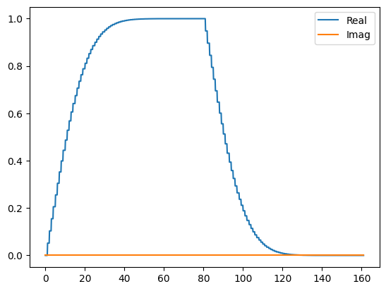
Observe, for example, the signal generated when all parameters are $10^{8}$ :

signal = signal_mapping(np.ones(80) * 1e8)
signal.draw(t0=0., tf=signal.duration * signal.dt, n=1000, function='envelope')

../_images/optimizing_pulse_sequence_3_0.png

4. Define gate fidelity#

We will optimize an $X$ gate, and define the fidelity of the unitary $U$ implemented by the pulse via the standard fidelity measure:

f (U) = \frac{| Tr (X U) |^{2}}{4}

X_op = Operator.from_label('X').data

def fidelity(U):
    return jnp.abs(jnp.sum(X_op * U))**2 / 4.

5. Define the objective function#

The function we want to optimize consists of:

Taking a list of input samples and applying the signal mapping.
Simulating the Schrodinger equation over the length of the pulse sequence.
Computing and return the infidelity (we minimize $1 - f (U)$ ).

def objective(params):

    # apply signal mapping and set signals
    signal = signal_mapping(params)

    # Simulate
    results = ham_solver.solve(
        y0=np.eye(2, dtype=complex),
        t_span=[0, signal.duration * signal.dt],
        signals=[signal],
        method='jax_odeint',
        atol=1e-8,
        rtol=1e-8
    )
    U = results.y[-1]

    # compute and return infidelity
    fid = fidelity(U)
    return 1. - fid

6. Perform JAX transformations and optimize#

Finally, we gradient optimize the objective:

Use jax.value_and_grad to transform the objective into a function that computes both the objective and the gradient.
Use jax.jit to just-in-time compile the function into optimized XLA code. For the initial cost of performing the compilation, this speeds up each call of the function, speeding up the optimization.
Call scipy.optimize.minimize with the above, with method='BFGS' and jac=True to indicate that the passed objective also computes the gradient.

from jax import jit, value_and_grad
from scipy.optimize import minimize

jit_grad_obj = jit(value_and_grad(objective))

initial_guess = np.random.rand(80) - 0.5

opt_results = minimize(fun=jit_grad_obj, x0=initial_guess, jac=True, method='BFGS')
print(opt_results.message)
print('Number of function evaluations: ' + str(opt_results.nfev))
print('Function value: ' + str(opt_results.fun))

Optimization terminated successfully.
Number of function evaluations: 12
Function value: -6.07233219263037e-08

The gate is optimized to an $X$ gate, with deviation within the numerical accuracy of the solver.

We can draw the optimized signal, which is retrieved by applying the signal_mapping to the optimized parameters.

opt_signal = signal_mapping(opt_results.x)

opt_signal.draw(
    t0=0,
    tf=opt_signal.duration * opt_signal.dt,
    n=1000,
    function='envelope',
    title='Optimized envelope'
)

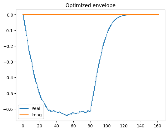
../_images/optimizing_pulse_sequence_7_0.png

Summing the signal samples yields approximately $\pm 50$ , which is equivalent to what one would expect based on a rotating wave approximation analysis.

opt_signal.samples.sum()

Array(50.00040529, dtype=float64)

7. Repeat the $X$ -gate optimization, alternatively using pulse schedules to specify the control sequence#

Here, we perform the optimization again, however now we specify the parameterized control sequence to optimize as a pulse schedule.

We construct a Gaussian square pulse as a ScalableSymbolicPulse instance, parameterized by sigma and width. Although qiskit pulse provides a GaussianSquare, this class is not JAX compatible. See the user guide entry on JAX-compatible pulse schedules.

import sympy as sym
from qiskit import pulse

def lifted_gaussian(
    t: sym.Symbol,
    center,
    t_zero,
    sigma,
) -> sym.Expr:
    t_shifted = (t - center).expand()
    t_offset = (t_zero - center).expand()

    gauss = sym.exp(-((t_shifted / sigma) ** 2) / 2)
    offset = sym.exp(-((t_offset / sigma) ** 2) / 2)

    return (gauss - offset) / (1 - offset)

def gaussian_square_generated_by_pulse(params):

    sigma, width = params
    _t, _duration, _amp, _sigma, _width, _angle = sym.symbols(
        "t, duration, amp, sigma, width, angle"
    )
    _center = _duration / 2

    _sq_t0 = _center - _width / 2
    _sq_t1 = _center + _width / 2

    _gaussian_ledge = lifted_gaussian(_t, _sq_t0, -1, _sigma)
    _gaussian_redge = lifted_gaussian(_t, _sq_t1, _duration + 1, _sigma)

    envelope_expr = (
        _amp
        * sym.exp(sym.I * _angle)
        * sym.Piecewise(
            (_gaussian_ledge, _t <= _sq_t0), (_gaussian_redge, _t >= _sq_t1), (1, True)
        )
    )

    # we need to set disable_validation True to enable jax-jitting.
    pulse.ScalableSymbolicPulse.disable_validation = True

    return pulse.ScalableSymbolicPulse(
            pulse_type="GaussianSquare",
            duration=230,
            amp=1,
            angle=0,
            parameters={"sigma": sigma, "width": width},
            envelope=envelope_expr,
            constraints=sym.And(_sigma > 0, _width >= 0, _duration >= _width),
            valid_amp_conditions=sym.Abs(_amp) <= 1.0,
        )

Next, we construct a pulse schedule using the above parametrized Gaussian square pulse, convert it to a signal, and simulate the equation over the length of the pulse sequence.

from qiskit_dynamics.pulse import InstructionToSignals

dt = 0.222
w = 5.

def objective(params):

    instance = gaussian_square_generated_by_pulse(params)

    with pulse.build() as Xp:
        pulse.play(instance, pulse.DriveChannel(0))

    converter = InstructionToSignals(dt, carriers={"d0": w})
    signal = converter.get_signals(Xp)

    result = ham_solver.solve(
        y0=np.eye(2, dtype=complex),
        t_span=[0, instance.duration * dt],
        signals=[signal],
        method='jax_odeint',
        atol=1e-8,
        rtol=1e-8
    )
    return 1. - fidelity(result[0].y[-1])

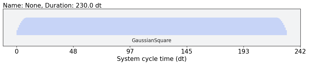
We set the initial values of sigma and width for the optimization as initial_params = np.array([10, 10]).

initial_params = np.array([10, 10])
gaussian_square_generated_by_pulse(initial_params).draw()

../_images/optimizing_pulse_sequence_11_0.png

from jax import jit, value_and_grad
from scipy.optimize import minimize

jit_grad_obj = jit(value_and_grad(objective))

initial_params = np.array([10,10])


opt_results = minimize(fun=jit_grad_obj, x0=initial_params, jac=True, method='BFGS')

print(opt_results.message)
print(f"Optimized Sigma is {opt_results.x[0]} and Width is {opt_results.x[1]}")
print('Number of function evaluations: ' + str(opt_results.nfev))
print('Function value: ' + str(opt_results.fun))

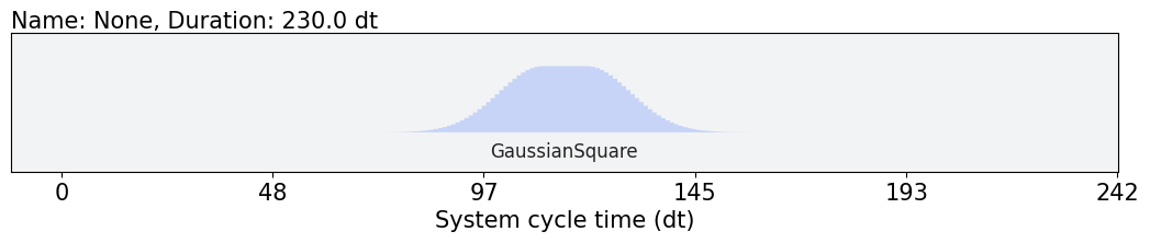
Optimization terminated successfully.
Optimized Sigma is 516.3449186228395 and Width is 212.18189863023863
Number of function evaluations: 14
Function value: 1.7537254681787573e-07

We can draw the optimized pulse, whose parameters are retrieved by opt_results.x.

gaussian_square_generated_by_pulse(opt_results.x).draw()

../_images/optimizing_pulse_sequence_13_0.png