Fermionic fast Fourier transform

The discrete Fourier transform on fermionic creation operators is defined as:

\[a^\dagger_k \mapsto \frac{1}{\sqrt{N}} \sum_{n=0}^{N-1} e^{-i 2\pi k n / N} a^\dagger_n\]

This is an orbital rotation whose matrix is the unitary DFT matrix \(F_N\) with entries \((F_N)_{kn} = \omega_N^{kn} / \sqrt{N}\), where \(\omega_N = e^{-i 2\pi / N}\). Rather than decomposing \(F_N\) directly into Givens rotations, the fermionic fast Fourier transform (FFFT) uses the Cooley-Tukey algorithm to break it into DFTs of prime size.

Mixed-radix Cooley-Tukey algorithm

The circuit follows the general factorization described in the Variations section of the Cooley-Tukey FFT algorithm Wikipedia page. First, \(N\) is factored into primes using trial division (this is the simple method, which might be improved in future). Writing \(N = N_1 N_2\), where \(N_2\) is the smallest prime factor, and splitting the input index as \(n = N_1 n_2 + n_1\) and the output index as \(k = N_2 k_1 + k_2\), the DFT becomes

\[X_{N_2 k_1 + k_2} = \sum_{n_1=0}^{N_1-1} \left[ e^{-\frac{2\pi i}{N_1N_2} n_1 k_2 } \right] \left( \sum_{n_2=0}^{N_2-1} x_{N_1 n_2 + n_1} e^{-\frac{2\pi i}{N_2} n_2 k_2 } \right) e^{-\frac{2\pi i}{N_1} n_1 k_1 }\]

where each inner sum is a DFT of size \(N_2\), each outer sum is a DFT of size \(N_1\).

The circuit follows this formula:

1. Perform \(N_1\) DFTs of size \(N_2\), one for each \(n_1\) (the inner sum). Since \(N_2\) is prime, each is implemented directly as an orbital rotation.

2. Multiply by the twiddle factors \(e^{-\frac{2\pi i}{N_1N_2} n_1 k_2 }\). Each twiddle factor multiplies a single mode, so it is implemented with a single-qubit phase gate.

3. Perform \(N_2\) DFTs of size \(N_1\), one for each \(k_2\) (the outer sum). These are computed by applying the same procedure recursively.

The recursion ends when the size is prime, in which case the DFT is implemented directly as an orbital rotation.

Under the Jordan-Wigner transformation, a gate implementing an orbital rotation must act on a contiguous block of qubits, because a hopping term between two modes carries a string of \(Z\) operators on all the qubits in between. The DFTs in steps 1 and 3 act on strided subsets of modes, so the circuit inserts fermionic mode permutations (themselves orbital rotations by permutation matrices) that bring each subset onto adjacent qubits before the DFTs are applied.

Quantum circuit implementation

Under the Jordan-Wigner transformation, FermionicFFTSpinlessJW and FermionicFFTJW construct quantum circuits for single-spin and spinful systems, respectively.

The following code cell constructs and displays a Qiskit circuit for implementing the fermionic fast Fourier transform on \(N = 6\) spatial orbitals, so \(N_2 = 2\) and \(N_1 = 3\). In the decomposed circuit you can see the mode permutations, the three size-2 DFTs of step 1 and the two size-3 DFTs of step 3 (as orbital rotations), and the twiddle-factor phase gates of step 2.

from qiskit.circuit import QuantumCircuit, QuantumRegister

import ffsim

norb = 6

# Spinless FFFT circuit (acts on norb qubits)
qubits = QuantumRegister(norb, name="q")
circuit = QuantumCircuit(qubits)
circuit.append(ffsim.qiskit.FermionicFFTSpinlessJW(norb), qubits)

# Decompose and draw
circuit.decompose().draw("mpl", scale=0.6)

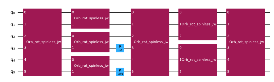
We can check that the circuit implements the DFT orbital rotation by comparing it against ffsim.apply_orbital_rotation with the DFT matrix on a random state.

import numpy as np
import scipy.linalg
from qiskit.quantum_info import Statevector

nocc = 3
nelec = (nocc, 0)
vec = ffsim.random.random_state_vector(ffsim.dim(norb, nelec), seed=1234)

# Apply the FFFT circuit to the state
qiskit_vec = ffsim.qiskit.ffsim_vec_to_qiskit_vec(vec, norb=norb, nelec=nelec)
result = Statevector(qiskit_vec).evolve(circuit)
result = ffsim.qiskit.qiskit_vec_to_ffsim_vec(np.array(result), norb=norb, nelec=nelec)

# Apply the DFT matrix as an orbital rotation
dft_mat = scipy.linalg.dft(norb, scale="sqrtn")
expected = ffsim.apply_orbital_rotation(vec, dft_mat, norb=norb, nelec=nelec)

np.allclose(result, expected)

True

For spinful systems across \(2 \times \text{norb}\) qubits, FermionicFFTJW applies independent sub-circuits for spin alpha (first norb qubits) and spin beta (last norb qubits).

norb = 4
nelec = (2, 2)  # 2 alpha electrons, 2 beta electrons

qubits = QuantumRegister(2 * norb, name="q")
circuit = QuantumCircuit(qubits)
circuit.append(ffsim.qiskit.PrepareHartreeFockJW(norb, nelec), qubits)
circuit.append(ffsim.qiskit.FermionicFFTJW(norb), qubits)

circuit.decompose().draw("mpl", scale=0.6)

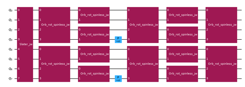
Cost compared with a direct orbital rotation

The DFT could also be implemented as a single orbital rotation by passing the DFT matrix to OrbitalRotationSpinlessJW, which decomposes it directly into Givens rotations. The following code cell compiles both circuits to a basis of CX, \(R_Z\), and Clifford single-qubit gates. For each one it reports the number of CX gates, the number of \(R_Z\) rotations whose angle is not a multiple of \(\pi/2\) (that is, the non-Clifford rotations), and how many distinct angles those rotations use, each as FFFT / direct.

import math

from qiskit import transpile

basis_gates = ["cx", "rz", "h", "s", "sdg", "x", "sx"]


def cost(gate) -> tuple[int, int, int]:
    """Return CX count, non-Clifford Rz count, and number of distinct angles."""
    circuit = QuantumCircuit(gate.num_qubits)
    circuit.append(gate, range(gate.num_qubits))
    transpiled = transpile(circuit, basis_gates=basis_gates, optimization_level=1)
    angles = []
    for instruction in transpiled.data:
        if instruction.operation.name == "rz":
            angle = float(instruction.operation.params[0]) % (2 * math.pi)
            remainder = angle % (math.pi / 2)
            if min(remainder, math.pi / 2 - remainder) > 1e-8:
                angles.append(round(angle, 8))
    return transpiled.count_ops().get("cx", 0), len(angles), len(set(angles))


print(f"{'N':>3} {'CX':>11} {'non-Clifford Rz':>17} {'distinct angles':>17}")
for n in [4, 8, 16, 6, 12]:
    ffft = cost(ffsim.qiskit.FermionicFFTSpinlessJW(n))
    direct = cost(
        ffsim.qiskit.OrbitalRotationSpinlessJW(n, scipy.linalg.dft(n, scale="sqrtn"))
    )
    cx, rz, angles = (f"{f} / {d}" for f, d in zip(ffft, direct))
    print(f"{n:>3} {cx:>11} {rz:>17} {angles:>17}")

  N          CX   non-Clifford Rz   distinct angles
  4     28 / 24            8 / 18             1 / 6
  8   144 / 112          26 / 111            2 / 58
 16   656 / 480          74 / 479           5 / 226
  6     72 / 60           34 / 60            8 / 31
 12   348 / 264          84 / 263           8 / 129

The FFFT needs far fewer non-Clifford rotations than the direct orbital rotation, and those rotations use only a handful of distinct angles. This is most pronounced when \(N\) is a power of 2. Then every Givens rotation is either a mode permutation (angle \(\pi/2\)) or a DFT of size 2 (angle \(\pi/4\)), and the only other angles come from twiddle factors, which are multiples of \(2\pi/N\). The direct orbital rotation, by contrast, needs a generic angle for almost every rotation. On fault-tolerant hardware, where each arbitrary-angle rotation must be synthesized from many expensive non-Clifford gates, this makes the FFFT much cheaper.

The price is more CX gates, since the mode permutations add two-qubit gates that the direct decomposition doesn’t need. When CX count is the main cost, as on current noisy hardware, the direct orbital rotation is the better choice.