Orbital rotations
The orbital rotation is a fundamental operation in the simulation of fermions. This page discusses orbital rotations and their properties.
Definition of orbital rotation
An orbital rotation is described by an \(N \times N\) unitary matrix \(\mathbf{U}\) (here \(N\) is the number spatial orbitals), and we denote the corresponding operator as \(\mathcal{U}\). This operator has the following action on the fermionic creation operators \(\set{a^\dagger_{i\sigma}}\):
That is, \(a^\dagger_{i\sigma}\) is mapped to a new operator \(b^\dagger_{i\sigma}\) where \(b^\dagger_{i\sigma}\) is a linear combination of the operators \(\set{a^\dagger_{i\sigma}}\) with coefficients given by the \(i\)-th column of \(\mathbf{U}\). The fact that \(\mathbf{U}\) is unitary can be used, together with the fermionic anticommutation relations, to show that the \(\set{b^\dagger_{i\sigma}}\) also satisfy the fermionic anticommutation relations. Thus, the \(b^\dagger_{i\sigma}\) are creation operators in a rotated basis of orbitals.
Explicit expression
It is a theorem that \(\mathcal{U}\) can be written explicitly as
Sometimes, it is useful to specify the orbital rotation via the antihermitian matrix \(\mathbf{K} = \log(\mathbf{U})\) rather than \(\mathbf{U}\) itself. However, ffsim generally represents orbital rotations using the unitary matrix \(\mathbf{U}\).
Homomorphism property
The mapping \(\mathbf{U} \mapsto \mathcal{U}\) satisfies the important homomorphism property:
for any unitary matrices \(\mathbf{U}\), \(\mathbf{U}_1\), and \(\mathbf{U}_2\).
Independent orbital rotations for spin-up and spin-down
The definitions given above assume that the same orbital rotation applies to both the spin-up and spin-down orbitals. However, it is possible for each spin sector to have an independent orbital rotation, in which case a pair of unitary matrices \((\mathbf{U}^\alpha, \mathbf{U}^\beta)\) needs to be specified. Letting \(\mathbf{K}^\sigma = \log(\mathbf{U}^\sigma)\), the definitions above then become
Application to time evolution by a quadratic Hamiltonian
A quadratic Hamiltonian is an operator of the form (here we restrict the definition to Hamiltonians with particle number and spin Z symmetry)
where \(\mathbf{M}\) is a Hermitian matrix. Time evolution by this Hamiltonian is given by the operator \(e^{-i \mathcal{M} t}\), where \(t\) is the evolution time. Orbital rotations can be used to implement time evolution by a quadratic Hamiltonian using two different methods.
Method 1: Diagonalize the quadratic Hamiltonian
A quadratic Hamiltonian can always be rewritten as
where the \(\set{\lambda_i}\) are real numbers called orbital energies, \(\mathcal{U}\) is an orbital rotation, and \(n_{i\sigma} = a^\dagger_{i\sigma} a_{i\sigma}\) is the occupation number operator. The \(\set{\lambda_i}\) and the unitary matrix \(\mathbf{U}\) describing the orbital rotation are obtained from an eigendecomposition of \(\mathbf{M}\):
Time evolution by \(\mathcal{M}\) can be implemented with the following steps:
Compute the orbital energies \(\set{\lambda_i}\) and the orbital rotation matrix \(\mathbf{U}\) by performing an eigendecomposition of \(\mathbf{M}\).
Perform the orbital rotation \(\mathcal{U}^\dagger\), which corresponds to the matrix \(\mathbf{U}^\dagger\).
Perform time evolution by the operator \(\sum_{i \sigma} \lambda_i n_{i\sigma}\).
Perform the orbital rotation \(\mathcal{U}^\dagger\), which corresponds to the matrix \(\mathbf{U}\).
Method 2: Implement directly as an orbital rotation
Reviewing the definition of an orbital rotation, we can see that the time evolution operator \(e^{-i \mathcal{M} t}\) is itself an orbital rotation defined by \(\mathbf{K} = -i \mathbf{M} t\), or \(\mathbf{U} = e^{-i \mathbf{M} t}\). Thus, the time evolution operator can be implemented directly as an orbital rotation.
The following code cell demonstrates the equivalence of the two methods by applying them to a randomly generated state vector and checking that the result is the same in both cases.
[1]:
import numpy as np
import scipy.linalg

import ffsim

rng = np.random.default_rng(12345)
norb = 6
nelec = (3, 3)

# Generate a random Hermitian matrix M to represent the quadratic Hamiltonian
mat = ffsim.random.random_hermitian(norb, seed=rng)

# Generate a random state vector and set the evolution time
vec = ffsim.random.random_state_vector(ffsim.dim(norb, nelec), seed=rng)
time = 1.0

# Apply time evolution via diagonalization
eigs, orbital_rotation = scipy.linalg.eigh(mat)
result1 = ffsim.apply_num_op_sum_evolution(
    vec, eigs, time=time, norb=norb, nelec=nelec, orbital_rotation=orbital_rotation
)

# Apply time evolution directly as an orbital rotation
evolution_mat = scipy.linalg.expm(-1j * time * mat)
result2 = ffsim.apply_orbital_rotation(vec, evolution_mat, norb=norb, nelec=nelec)

# Check that the results match
np.testing.assert_allclose(result1, result2)
The apply_quad_ham_evolution function implements time evolution by a quadratic Hamiltonian. Internally, it implements the evolution directly as an orbital rotation (Method 2).
[2]:
result3 = ffsim.apply_quad_ham_evolution(vec, mat, time, norb=norb, nelec=nelec)

np.testing.assert_allclose(result3, result1)
Quantum circuit implementation
An orbital rotation can be implemented as a quantum circuit by decomposing it into Givens rotations. Under the Jordan-Wigner transformation, the circuit can be implemented as a dense brickwork pattern of two-qubit rotations, followed by a single layer of single-qubit phase gates. The following code cell constructs and displays a Qiskit circuit for implementing an orbital rotation. Notice that the circuit consists of two independent sub-circuits acting on each spin sector.
[3]:
from qiskit.circuit import QuantumCircuit, QuantumRegister

norb = 6
nelec = (3, 3)

# Generate a random orbital rotation
orbital_rotation = ffsim.random.random_unitary(norb, seed=rng)

# Create a quantum circuit that implements this orbital rotation
qubits = QuantumRegister(2 * norb, name="q")
circuit = QuantumCircuit(qubits)
circuit.append(ffsim.qiskit.OrbitalRotationJW(norb, orbital_rotation), qubits)

# Decompose the orbital rotation into basic gates before drawing
circuit.decompose().draw("mpl", scale=0.6)
[3]:

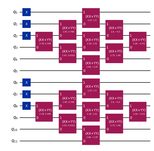
When an orbital rotation is applied to a single electronic configuration (in the qubit picture, a computational basis state), the quantum circuit implementation can be optimized to use fewer gates, resulting in a “diamond” pattern of gates rather than a dense “brickwork” pattern. For additional information, see Jiang et al. (2018).
The following code cell constructs and displays an example of the optimized circuit.
[4]:
# Create a quantum circuit that applies an orbital rotation to the Hartree-Fock state
circuit = QuantumCircuit(qubits)
circuit.append(ffsim.qiskit.PrepareHartreeFockJW(norb, nelec), qubits)
circuit.append(ffsim.qiskit.OrbitalRotationJW(norb, orbital_rotation), qubits)

# Optimize the orbital rotation circuit
circuit = ffsim.qiskit.PRE_INIT.run(circuit)

# Decompose the orbital rotation into basic gates before drawing
circuit.decompose().draw("mpl", scale=0.6)
[4]: