Quantum State Tomography

Quantum tomography is an experimental procedure to reconstruct a description of part of a quantum system from the measurement outcomes of a specific set of experiments. In particular, quantum state tomography reconstructs the density matrix of a quantum state by preparing the state many times and measuring them in a tomographically complete basis of measurement operators.

Note

This tutorial requires the qiskit-aer and qiskit-ibm-runtime packages to run simulations. You can install them with python -m pip install qiskit-aer qiskit-ibm-runtime.

We first initialize a simulator to run the experiments on.

from qiskit_aer import AerSimulator
from qiskit_ibm_runtime.fake_provider import FakePerth

backend = AerSimulator.from_backend(FakePerth())

To run a state tomography experiment, we initialize the experiment with a circuit to prepare the state to be measured. We can also pass in an Operator or a Statevector to describe the preparation circuit.

import qiskit
from qiskit_experiments.framework import ParallelExperiment
from qiskit_experiments.library import StateTomography

# GHZ State preparation circuit
nq = 2
qc_ghz = qiskit.QuantumCircuit(nq)
qc_ghz.h(0)
qc_ghz.s(0)
for i in range(1, nq):
    qc_ghz.cx(0, i)

# QST Experiment
qstexp1 = StateTomography(qc_ghz)
qstdata1 = qstexp1.run(backend, seed_simulation=100).block_for_results()

# Print results
for result in qstdata1.analysis_results():
    print(result)

AnalysisResult
- name: state
- value: DensityMatrix([[ 0.46809896+0.00000000e+00j,  0.01660156-8.78906250e-03j,
                 0.00537109+7.16145833e-03j,  0.00830078-4.40429688e-01j],
               [ 0.01660156+8.78906250e-03j,  0.03385417+0.00000000e+00j,
                -0.00146484+3.90625000e-03j, -0.00439453+4.23177083e-03j],
               [ 0.00537109-7.16145833e-03j, -0.00146484-3.90625000e-03j,
                 0.02864583+0.00000000e+00j, -0.01464844+3.46944695e-18j],
               [ 0.00830078+4.40429688e-01j, -0.00439453-4.23177083e-03j,
                -0.01464844-3.46944695e-18j,  0.46940104+0.00000000e+00j]],
              dims=(2, 2))
- quality: unknown
- extra: <9 items>
- device_components: ['Q0', 'Q1']
- verified: False
AnalysisResult
- name: state_fidelity
- value: 0.9091796874999994
- quality: unknown
- extra: <9 items>
- device_components: ['Q0', 'Q1']
- verified: False
AnalysisResult
- name: positive
- value: True
- quality: unknown
- extra: <9 items>
- device_components: ['Q0', 'Q1']
- verified: False

Tomography Results

The main result for tomography is the fitted state, which is stored as a DensityMatrix object:

state_result = qstdata1.analysis_results("state")
print(state_result.value)

DensityMatrix([[ 0.46809896+0.00000000e+00j,  0.01660156-8.78906250e-03j,
                 0.00537109+7.16145833e-03j,  0.00830078-4.40429688e-01j],
               [ 0.01660156+8.78906250e-03j,  0.03385417+0.00000000e+00j,
                -0.00146484+3.90625000e-03j, -0.00439453+4.23177083e-03j],
               [ 0.00537109-7.16145833e-03j, -0.00146484-3.90625000e-03j,
                 0.02864583+0.00000000e+00j, -0.01464844+3.46944695e-18j],
               [ 0.00830078+4.40429688e-01j, -0.00439453-4.23177083e-03j,
                -0.01464844-3.46944695e-18j,  0.46940104+0.00000000e+00j]],
              dims=(2, 2))

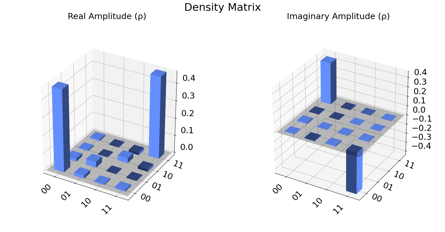
We can also visualize the density matrix:

from qiskit.visualization import plot_state_city
plot_state_city(qstdata1.analysis_results("state").value, title='Density Matrix')

The state fidelity of the fitted state with the ideal state prepared by the input circuit is stored in the "state_fidelity" result field. Note that if the input circuit contained any measurements the ideal state cannot be automatically generated and this field will be set to None.

fid_result = qstdata1.analysis_results("state_fidelity")
print("State Fidelity = {:.5f}".format(fid_result.value))

State Fidelity = 0.90918

Additional state metadata

Additional data is stored in the tomography under the "state_metadata" field. This includes

• eigvals: the eigenvalues of the fitted state

• trace: the trace of the fitted state

• positive: Whether the eigenvalues are all non-negative

• positive_delta: the deviation from positivity given by 1-norm of negative eigenvalues.

If trace rescaling was performed this dictionary will also contain a raw_trace field containing the trace before rescaling. Futhermore, if the state was rescaled to be positive or trace 1 an additional field raw_eigvals will contain the state eigenvalues before rescaling was performed.

state_result.extra

{'trace': 1.0000000000000016,
 'eigvals': array([0.90964207, 0.04920062, 0.03065617, 0.01050113]),
 'raw_eigvals': array([0.90964207, 0.04920062, 0.03065617, 0.01050113]),
 'rescaled_psd': False,
 'fitter_metadata': {'fitter': 'linear_inversion',
  'fitter_time': 0.0036745071411132812},
 'conditional_probability': 1.0,
 'positive': True,
 'experiment': 'StateTomography',
 'run_time': None}

To see the effect of rescaling, we can perform a “bad” fit with very low counts:

# QST Experiment
bad_data = qstexp1.run(backend, shots=10, seed_simulation=100).block_for_results()
bad_state_result = bad_data.analysis_results("state")

# Print result
print(bad_state_result)

# Show extra data
bad_state_result.extra

AnalysisResult
- name: state
- value: DensityMatrix([[ 0.53941247+0.00000000e+00j,  0.07448997-1.35224574e-02j,
                -0.10333108-3.24527629e-02j,  0.23016862-3.34916983e-01j],
               [ 0.07448997+1.35224574e-02j,  0.02987644+0.00000000e+00j,
                -0.01605575-2.68567164e-02j,  0.04583748-7.98356669e-02j],
               [-0.10333108+3.24527629e-02j, -0.01605575+2.68567164e-02j,
                 0.04243149+1.30104261e-18j,  0.0157413 +8.91334687e-02j],
               [ 0.23016862+3.34916983e-01j,  0.04583748+7.98356669e-02j,
                 0.0157413 -8.91334687e-02j,  0.38827961+0.00000000e+00j]],
              dims=(2, 2))
- quality: unknown
- extra: <9 items>
- device_components: ['Q0', 'Q1']
- verified: False

{'trace': 1.0000000000000013,
 'eigvals': array([0.91528963, 0.08471037, 0.        , 0.        ]),
 'raw_eigvals': array([ 0.97853197,  0.1479527 , -0.02024752, -0.10623715]),
 'rescaled_psd': True,
 'fitter_metadata': {'fitter': 'linear_inversion',
  'fitter_time': 0.003876209259033203},
 'conditional_probability': 1.0,
 'positive': True,
 'experiment': 'StateTomography',
 'run_time': None}

Tomography Fitters

The default fitters is linear_inversion, which reconstructs the state using dual basis of the tomography basis. This will typically result in a non-positive reconstructed state. This state is rescaled to be positive-semidefinite (PSD) by computing its eigen-decomposition and rescaling its eigenvalues using the approach from Ref. [1].

There are several other fitters are included (See API documentation for details). For example, if cvxpy is installed we can use the cvxpy_gaussian_lstsq() fitter, which allows constraining the fit to be PSD without requiring rescaling.

try:
    import cvxpy

    # Set analysis option for cvxpy fitter
    qstexp1.analysis.set_options(fitter='cvxpy_gaussian_lstsq')

    # Re-run experiment
    qstdata2 = qstexp1.run(backend, seed_simulation=100).block_for_results()

    state_result2 = qstdata2.analysis_results("state")
    print(state_result2)
    print("\nextra:")
    for key, val in state_result2.extra.items():
        print(f"- {key}: {val}")

except ModuleNotFoundError:
    print("CVXPY is not installed")

AnalysisResult
- name: state
- value: DensityMatrix([[ 4.87885248e-01+0.00000000e+00j,
                 4.16612970e-03+2.50168824e-04j,
                -4.06930842e-03+1.19437420e-02j,
                 8.37117905e-03-4.34678178e-01j],
               [ 4.16612970e-03-2.50168824e-04j,
                 1.98389136e-02+0.00000000e+00j,
                -1.05182900e-02+5.25257958e-03j,
                -2.35027214e-04-1.74903261e-03j],
               [-4.06930842e-03-1.19437420e-02j,
                -1.05182900e-02-5.25257958e-03j,
                 2.52179465e-02+0.00000000e+00j,
                -7.58397322e-04-4.68941354e-03j],
               [ 8.37117905e-03+4.34678178e-01j,
                -2.35027214e-04+1.74903261e-03j,
                -7.58397322e-04+4.68941354e-03j,
                 4.67057891e-01+0.00000000e+00j]],
              dims=(2, 2))
- quality: unknown
- extra: <9 items>
- device_components: ['Q0', 'Q1']
- verified: False

extra:
- trace: 1.0000000014177983
- eigvals: [0.91246964 0.04861046 0.0293311  0.0095888 ]
- raw_eigvals: [0.91246964 0.04861046 0.0293311  0.0095888 ]
- rescaled_psd: False
- fitter_metadata: {'fitter': 'cvxpy_gaussian_lstsq', 'cvxpy_solver': 'SCS', 'cvxpy_status': ['optimal'], 'psd_constraint': True, 'trace_preserving': True, 'fitter_time': 0.019322633743286133}
- conditional_probability: 1.0
- positive: True
- experiment: StateTomography
- run_time: None

Parallel Tomography Experiment

We can also use the ParallelExperiment class to run subsystem tomography on multiple qubits in parallel.

For example if we want to perform 1-qubit QST on several qubits at once:

from math import pi
num_qubits = 5
gates = [qiskit.circuit.library.RXGate(i * pi / (num_qubits - 1))
         for i in range(num_qubits)]

subexps = [
    StateTomography(gate, physical_qubits=(i,))
    for i, gate in enumerate(gates)
]
parexp = ParallelExperiment(subexps)
pardata = parexp.run(backend, seed_simulation=100).block_for_results()

for result in pardata.analysis_results():
    print(result)

AnalysisResult
- name: state
- value: DensityMatrix([[0.97363281+0.j        , 0.02050781-0.00195312j],
               [0.02050781+0.00195312j, 0.02636719+0.j        ]],
              dims=(2,))
- quality: unknown
- extra: <9 items>
- device_components: ['Q0']
- verified: False
AnalysisResult
- name: state_fidelity
- value: 0.9736328125000001
- quality: unknown
- extra: <9 items>
- device_components: ['Q0']
- verified: False
AnalysisResult
- name: positive
- value: True
- quality: unknown
- extra: <9 items>
- device_components: ['Q0']
- verified: False
AnalysisResult
- name: state
- value: DensityMatrix([[ 0.84667969+0.j        , -0.02246094+0.35058594j],
               [-0.02246094-0.35058594j,  0.15332031+0.j        ]],
              dims=(2,))
- quality: unknown
- extra: <9 items>
- device_components: ['Q1']
- verified: False
AnalysisResult
- name: state_fidelity
- value: 0.9930412517257765
- quality: unknown
- extra: <9 items>
- device_components: ['Q1']
- verified: False
AnalysisResult
- name: positive
- value: True
- quality: unknown
- extra: <9 items>
- device_components: ['Q1']
- verified: False
AnalysisResult
- name: state
- value: DensityMatrix([[ 0.50878906+0.j        , -0.02050781+0.46679688j],
               [-0.02050781-0.46679688j,  0.49121094+0.j        ]],
              dims=(2,))
- quality: unknown
- extra: <9 items>
- device_components: ['Q2']
- verified: False
AnalysisResult
- name: state_fidelity
- value: 0.9667968750000004
- quality: unknown
- extra: <9 items>
- device_components: ['Q2']
- verified: False
AnalysisResult
- name: positive
- value: True
- quality: unknown
- extra: <9 items>
- device_components: ['Q2']
- verified: False
AnalysisResult
- name: state
- value: DensityMatrix([[ 0.17285156+0.j        , -0.01269531+0.34765625j],
               [-0.01269531-0.34765625j,  0.82714844+0.j        ]],
              dims=(2,))
- quality: unknown
- extra: <9 items>
- device_components: ['Q3']
- verified: False
AnalysisResult
- name: state_fidelity
- value: 0.9771589705077196
- quality: unknown
- extra: <9 items>
- device_components: ['Q3']
- verified: False
AnalysisResult
- name: positive
- value: True
- quality: unknown
- extra: <9 items>
- device_components: ['Q3']
- verified: False
AnalysisResult
- name: state
- value: DensityMatrix([[ 0.03320313+0.j        , -0.00292969-0.01660156j],
               [-0.00292969+0.01660156j,  0.96679687+0.j        ]],
              dims=(2,))
- quality: unknown
- extra: <9 items>
- device_components: ['Q4']
- verified: False
AnalysisResult
- name: state_fidelity
- value: 0.9667968750000002
- quality: unknown
- extra: <9 items>
- device_components: ['Q4']
- verified: False
AnalysisResult
- name: positive
- value: True
- quality: unknown
- extra: <9 items>
- device_components: ['Q4']
- verified: False

View component experiment analysis results:

for i, expdata in enumerate(pardata.child_data()):
    state_result_i = expdata.analysis_results("state")
    fid_result_i = expdata.analysis_results("state_fidelity")

    print(f'\nPARALLEL EXP {i}')
    print("State Fidelity: {:.5f}".format(fid_result_i.value))
    print("State: {}".format(state_result_i.value))

References

[1]

J Smolin, JM Gambetta, G Smith, Phys. Rev. Lett. 108, 070502 (2012), open access.

See also

• API documentation: StateTomography