Braket-native primitives¶

In this notebook, we will learn how to use the BraketEstimator and BraketSampler primitives to run Qiskit workloads on Amazon Braket. Under the hood, these primitives run program sets with parametrized circuits and lists of input parameter values, which can be significantly more efficient than their BackendEstimator and BackendSampler counterparts, which bind the parameter values of the circuits first, resulting in a copy of a circuit for each of its input parameter values.

We begin by importing all required classes and functions.

[1]:

import matplotlib.pyplot as plt
import numpy as np
from qiskit.circuit import ClassicalRegister, Parameter, QuantumCircuit, QuantumRegister
from qiskit.quantum_info import SparsePauliOp

from qiskit_braket_provider import BraketEstimator, BraketLocalBackend, BraketSampler

BraketEstimator¶

An estimator primitive computes the expectation values of one or multiple observables with respect to states prepared by quantum circuits. The circuits may be parametrized, with input values specified alongside the circuit and observable. The BraketEstimator constructs and runs a program set from the given estimator PUBs, which are (circuit, observable, parameter (optional)) triplets.

[2]:

backend = BraketLocalBackend()
estimator = BraketEstimator(backend=backend)

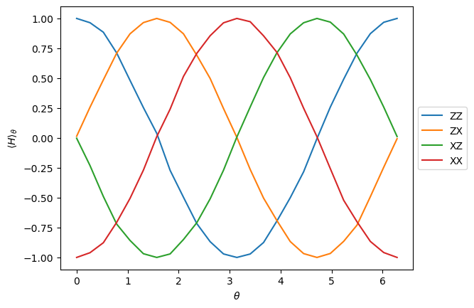
Now, let’s define a parametrized circuit with single parameter. We will measure this circuit with four observables and sweep through 25 parameter values:

[3]:

circuit = QuantumCircuit(2)
circuit.h(0)
circuit.cx(0, 1)
circuit.ry(Parameter("θ"), 0)

parameters = [[ph] for ph in np.linspace(0, 2 * np.pi, 25)]
observables = [
    [SparsePauliOp("ZZ")],
    [SparsePauliOp("ZX")],
    [SparsePauliOp("XZ")],
    [SparsePauliOp("XX", -1)],  # Multiply by -1 to distinguish from ZZ
]

estimator_pub = circuit, observables, parameters

We can then see how the expectation of each observable varies with the parameters:

[4]:

task = estimator.run([estimator_pub], precision=0.015625)
evs = task.result()[0].data.evs
fig = plt.figure()
plt.plot(parameters, evs[0], label="ZZ")
plt.plot(parameters, evs[1], "tab:orange", label="ZX")
plt.plot(parameters, evs[2], "tab:green", label="XZ")
plt.plot(parameters, evs[3], "tab:red", label="XX")
plt.xlabel(r"$\theta$")
plt.ylabel(r"$\langle H \rangle_\theta$")
fig.legend(loc="upper left", bbox_to_anchor=(0.9, 0.6))

[4]:

<matplotlib.legend.Legend at 0x311fcebc0>

../_images/tutorials_6_tutorial_primitives_7_1.png

The resulting program set consists of a single program with 100 executables from taking the Cartesian product of the observables and parameters.

[5]:

program_set = task.program_set
print(f"Number of programs: {len(program_set)}")
print(f"Number of executables: {len(program_set[0])}")

Number of programs: 1
Number of executables: 100

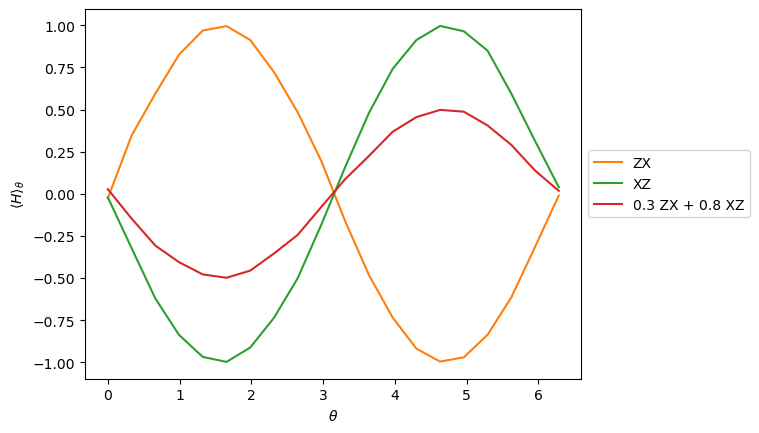
In the previous example, every observable was a single-term Pauli operator. However, observables can also be multi-term Hamiltonians:

[6]:

parameters = [[ph] for ph in np.linspace(0, 2 * np.pi, 20)]
observables = [
    [SparsePauliOp("ZX")],
    [SparsePauliOp("XZ")],
    [SparsePauliOp(["ZX", "XZ"], [0.3, 0.8])],
]

The red line shows the expectation value of the Hamiltonian, which is a linear combination of \(ZX\) (orange) and \(XZ\) (green):

[7]:

task = estimator.run([(circuit, observables, parameters)], precision=0.015625)
evs = task.result()[0].data.evs
fig = plt.figure()
plt.plot(parameters, evs[0], "tab:orange", label="ZX")
plt.plot(parameters, evs[1], "tab:green", label="XZ")
plt.plot(parameters, evs[2], "tab:red", label="0.3 ZX + 0.8 XZ")
plt.xlabel(r"$\theta$")
plt.ylabel(r"$\langle H \rangle_\theta$")
fig.legend(loc="upper left", bbox_to_anchor=(0.9, 0.6))

[7]:

<matplotlib.legend.Legend at 0x311fcd990>

../_images/tutorials_6_tutorial_primitives_13_1.png

Each Hamiltonian will get a dedicated program in the program set, and each term of the Hamiltonian will be a separate executable; as such, the PUB we just ran generates two programs:

[8]:

program_set = task.program_set
print(f"Number of programs: {len(program_set)}\n")
print(f"Hamiltonian in first program: {program_set[0].observables}")
print(f"Number of executables in first program: {len(program_set[0])}\n")
print(f"Observables in second program: {program_set[1].observables}")
print(f"Number of executables second program: {len(program_set[1])}")

Number of programs: 2

Hamiltonian in first program: Sum(TensorProduct(Z('qubit_count': 1, 'target': QubitSet([Qubit(0)])), X('qubit_count': 1, 'target': QubitSet([Qubit(1)]))), TensorProduct(X('qubit_count': 1, 'target': QubitSet([Qubit(0)])), Z('qubit_count': 1, 'target': QubitSet([Qubit(1)]))))
Number of executables in first program: 40

Observables in second program: [TensorProduct(X('qubit_count': 1, 'target': QubitSet([Qubit(0)])), Z('qubit_count': 1, 'target': QubitSet([Qubit(1)]))), TensorProduct(Z('qubit_count': 1, 'target': QubitSet([Qubit(0)])), X('qubit_count': 1, 'target': QubitSet([Qubit(1)])))]
Number of executables second program: 40

Note: Hamiltonian programs appear first in the list, but the order is corrected by the estimator’s postprocessing.

So far, we’ve only looked at examples where the observables and parameters are both 1-dimensional, which allows them to be paired in a Cartesian product. However, Qiskit allows observables and parameters to be of arbitrary shape, so long as they are broadcastable.

e1e9ebb7381445489525f5b26bdf11dc

Source: https://quantum.cloud.ibm.com/docs/en/guides/primitive-input-output#broadcasting-rules

Since programs in program sets only encode Cartesian products, a single PUB may require multiple programs to capture the full broadcasted combination:

[9]:

circuit = QuantumCircuit(2)
circuit.h(0)
circuit.cx(0, 1)
circuit.ry(Parameter("theta"), 0)
circuit.rz(Parameter("phi"), 0)
circuit.cx(0, 1)
circuit.h(0)

parameter_values = np.stack(  # shape (3, 6)
    [
        np.array(
            [np.linspace(-np.pi, np.pi, 6), np.linspace(-np.pi, 0, 6), np.linspace(0, np.pi / 2, 6)]
        ),
        np.array(
            [
                np.linspace(-4 * np.pi, 4 * np.pi, 6),
                np.linspace(-4 * np.pi, 0, 6),
                np.linspace(0, 4 * np.pi / 2, 6),
            ]
        ),
    ],
    axis=-1,
)
observables = [  # shape (2, 3, 1)
    [
        [SparsePauliOp(["XX", "IY"], [0.5, 0.5])],
        [SparsePauliOp("XX")],
        [SparsePauliOp("IY")],
    ],
    [
        [SparsePauliOp("ZZ")],
        [SparsePauliOp(["ZZ", "IX"], [0.5, 0.5])],
        [SparsePauliOp("IX")],
    ],
]

We see that the shape of the result is the broadcasted shape of the observables and parameters:

[10]:

task = estimator.run([(circuit, observables, parameter_values)], precision=0.015625)
evs = task.result()[0].data.evs
evs.shape

[10]:

(2, 3, 6)

In the (2, 3, 6) array in the diagram above, the broadcasted array is shown as two sheets standing back-to-back, where each sheet has different observables. However, the array can also be interpreted as a vertical stack of three “layers”, where each layer shares the same parameter values; this second interpretation is how the Cartesian products are “sliced out” in the program set.

The top layer gets two programs, one for the Hamiltonian and one for the monomial
The same goes for the middle layer
The bottom layer gets a single program because both observables are monomials

[11]:

program_set = task.program_set
print(f"Number of programs: {len(program_set)}\n")
print(f"Hamiltonian in first program: {program_set[0].observables}")
print(f"Observables in second program: {program_set[1].observables}")
print(f"Hamiltonian in third program: {program_set[2].observables}")
print(f"Observables in fourth program: {program_set[3].observables}")
print(f"Observables in fifth program: {program_set[4].observables}")

Number of programs: 5

Hamiltonian in first program: Sum(Y('qubit_count': 1, 'target': QubitSet([Qubit(0)])), TensorProduct(X('qubit_count': 1, 'target': QubitSet([Qubit(0)])), X('qubit_count': 1, 'target': QubitSet([Qubit(1)]))))
Observables in second program: [TensorProduct(Z('qubit_count': 1, 'target': QubitSet([Qubit(0)])), Z('qubit_count': 1, 'target': QubitSet([Qubit(1)])))]
Hamiltonian in third program: Sum(X('qubit_count': 1, 'target': QubitSet([Qubit(0)])), TensorProduct(Z('qubit_count': 1, 'target': QubitSet([Qubit(0)])), Z('qubit_count': 1, 'target': QubitSet([Qubit(1)]))))
Observables in fourth program: [TensorProduct(X('qubit_count': 1, 'target': QubitSet([Qubit(0)])), X('qubit_count': 1, 'target': QubitSet([Qubit(1)])))]
Observables in fifth program: [Y('qubit_count': 1, 'target': QubitSet([Qubit(0)])), X('qubit_count': 1, 'target': QubitSet([Qubit(0)]))]

BraketSampler¶

The sampler primitive samples the output of one or more quantum circuits, which may be parametrized if the input values are specified as well.

[12]:

sampler = BraketSampler(backend=backend)

As with the estimator, the parameters can be of any shape, and the results of running a sampler pub (circuit, parameters) will be of the same shape as the parameter array. We now run a 12-qubit version of the circuit from the first estimator example:

[13]:

circuit = QuantumCircuit(
    QuantumRegister(3, "qreg_a"),
    QuantumRegister(9, "qreg_b"),
    ClassicalRegister(10, "creg_a"),
    ClassicalRegister(2, "creg_b"),
)
circuit.h(0)
for i in range(11):
    circuit.cx(i, i + 1)
circuit.ry(Parameter("θ"), 0)
circuit.measure_all(add_bits=False)
parameter_values = np.array(  # shape (3, 7)
    [np.linspace(0, 2 * np.pi, 7), np.linspace(0, np.pi, 7), np.linspace(np.pi, 2 * np.pi, 7)]
)

result = sampler.run([(circuit, parameter_values)], shots=1024).result()
data = result[0].data
data.shape

/Users/caw/Documents/GitHub/qiskit-braket-provider/qiskit_braket_provider/providers/adapter.py:860: UserWarning: The Qiskit circuit contains barrier instructions that are ignored.
  warnings.warn("The Qiskit circuit contains barrier instructions that are ignored.")

[13]:

(3, 7)

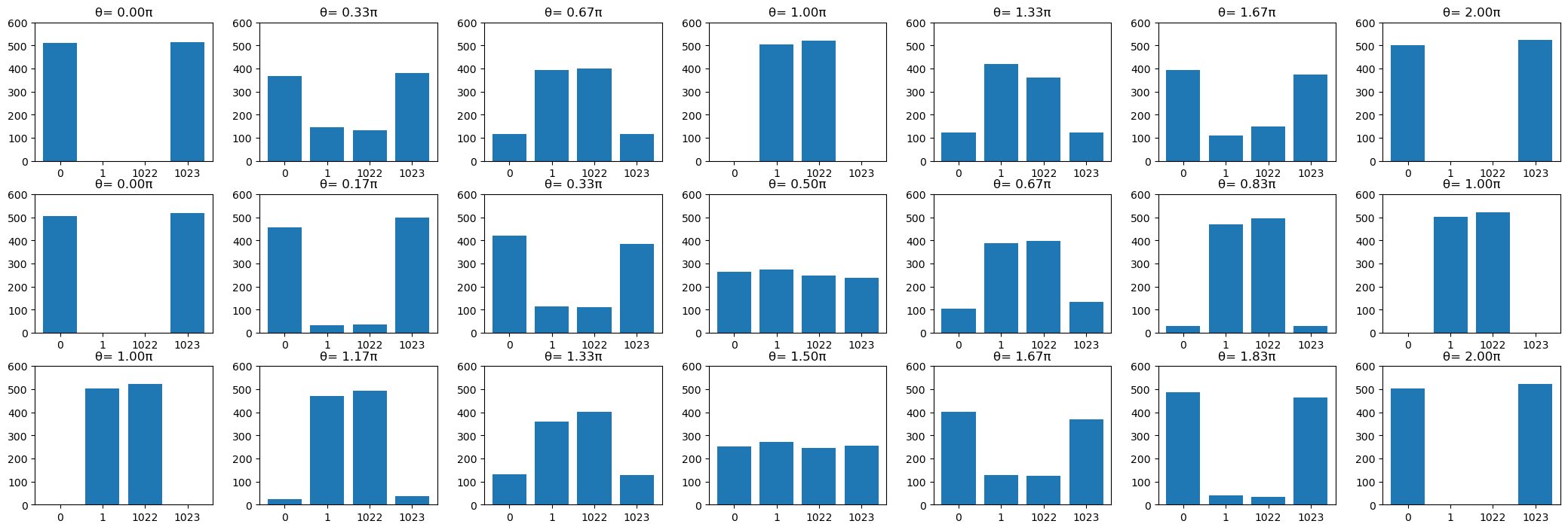
Looking at the first classical register, we see that its (marginal) probability distribution varies over \(\theta\) as

\[\mathbfit{p}(\theta) = \frac{1}{2} \left( \cos^2(\theta),\, \sin^2(\theta),\, 0, \cdots,\, 0,\, \sin^2(\theta),\, \cos^2(\theta) \right)\]

[14]:

fig, axs = plt.subplots(3, 7, figsize=(21, 7))
fig.tight_layout()
for index in np.ndindex(data.shape):
    x = []
    y = []
    counts = dict(data.creg_a[index].get_int_counts())
    for i in {0, 1, 1022, 1023}:
        counts.setdefault(i, 0)
    for k, v in sorted(counts.items()):
        x.append(str(k))
        y.append(v)
    axs[index].bar(x, y)
    axs[index].set_ylim(0, 600)
    axs[index].set_title(f"θ={round(parameter_values[index] * 6 / np.pi) / 6: .2f}π")

../_images/tutorials_6_tutorial_primitives_27_0.png