Minimum Eigen Optimizer
About this notebook and the adaptation to the Braket backend
The original version of this notebook is accessible at docs/tutorials/03_minimum_eigen_optimizer.ipynb. The only changes made to the original notebook are contained in the first cell and in cell #6 where we pass the BackendSampler object to execute the tasks on Amazon Braket SV1 simulator.
[1]:
from qiskit_braket_provider import BraketLocalBackend, BraketSampler

sampler = BraketSampler(BraketLocalBackend())
Introduction
An interesting class of optimization problems to be addressed by quantum computing are Quadratic Unconstrained Binary Optimization (QUBO) problems. Finding the solution to a QUBO is equivalent to finding the ground state of a corresponding Ising Hamiltonian, which is an important problem not only in optimization, but also in quantum chemistry and physics. For this translation, the binary variables taking values in \(\{0, 1\}\) are replaced by spin variables taking values in \(\{-1, +1\}\), which allows one to replace the resulting spin variables by Pauli Z matrices, and thus, an Ising Hamiltonian. For more details on this mapping we refer to [1].
Qiskit optimization provides automatic conversion from a suitable QuadraticProgram to an Ising Hamiltonian, which then allows leveraging all the SamplingMinimumEigensolver implementations, such as
SamplingVQE,QAOA, orNumpyMinimumEigensolver(classical exact method).
Note 1: MinimumEigenOptimizer does not support qiskit_algorithms.VQE. But qiskit_algorithms.SamplingVQE can be used instead.
Note 2: MinimumEigenOptimizer can use NumpyMinimumEigensolver as an exception case though it inherits MinimumEigensolver (not SamplingMinimumEigensolver).
Qiskit optimization provides a the MinimumEigenOptimizer class, which wraps the translation to an Ising Hamiltonian (in Qiskit Terra also called SparsePauliOp), the call to a MinimumEigensolver, and the translation of the results back to an OptimizationResult.
In the following we first illustrate the conversion from a QuadraticProgram to a SparsePauliOp and then show how to use the MinimumEigenOptimizer with different MinimumEigensolvers to solve a given QuadraticProgram. The algorithms in Qiskit optimization automatically try to convert a given problem to the supported problem class if possible, for instance, the MinimumEigenOptimizer will automatically translate integer variables to binary variables or add linear equality
constraints as a quadratic penalty term to the objective. It should be mentioned that a QiskitOptimizationError will be thrown if conversion of a quadratic program with integer variables is attempted.
The circuit depth of QAOA potentially has to be increased with the problem size, which might be prohibitive for near-term quantum devices. A possible workaround is Recursive QAOA, as introduced in [2]. Qiskit optimization generalizes this concept to the RecursiveMinimumEigenOptimizer, which is introduced at the end of this tutorial.
References
[1] A. Lucas, Ising formulations of many NP problems, Front. Phys., 12 (2014).
Converting a QUBO to a SparsePauliOp
[2]:
import numpy as np
from qiskit.visualization import plot_histogram
from qiskit_optimization import QuadraticProgram
from qiskit_optimization.algorithms import (
    MinimumEigenOptimizer,
    OptimizationResultStatus,
    RecursiveMinimumEigenOptimizer,
    SolutionSample,
)
from qiskit_optimization.minimum_eigensolvers import QAOA, NumPyMinimumEigensolver
from qiskit_optimization.optimizers import COBYLA
from qiskit_optimization.utils import algorithm_globals
/Users/caw/anaconda3/lib/python3.10/site-packages/pandas/core/arrays/masked.py:61: UserWarning: Pandas requires version '1.3.6' or newer of 'bottleneck' (version '1.3.5' currently installed).
  from pandas.core import (
[3]:
# create a QUBO
qubo = QuadraticProgram()
qubo.binary_var("x")
qubo.binary_var("y")
qubo.binary_var("z")
qubo.minimize(linear=[1, -2, 3], quadratic={("x", "y"): 1, ("x", "z"): -1, ("y", "z"): 2})
print(qubo.prettyprint())
Problem name:

Minimize
  x*y - x*z + 2*y*z + x - 2*y + 3*z

Subject to
  No constraints

  Binary variables (3)
    x y z
Next we translate this QUBO into an Ising operator. This results not only in a SparsePauliOp but also in a constant offset to be taken into account to shift the resulting value.
[4]:
op, offset = qubo.to_ising()
print(f"offset: {offset}")
print("operator:")
print(op)
offset: 1.5
operator:
SparsePauliOp(['IIZ', 'IZI', 'ZII', 'IZZ', 'ZIZ', 'ZZI'],
              coeffs=[-0.5 +0.j,  0.25+0.j, -1.75+0.j,  0.25+0.j, -0.25+0.j,  0.5 +0.j])
Sometimes a QuadraticProgram might also directly be given in the form of a SparsePauliOp. For such cases, Qiskit optimization also provides a translator from a SparsePauliOp back to a QuadraticProgram, which we illustrate in the following.
[5]:
qp = QuadraticProgram()
qp.from_ising(op, offset, linear=True)
print(qp.prettyprint())
Problem name:

Minimize
  x0*x1 - x0*x2 + 2*x1*x2 + x0 - 2*x1 + 3*x2

Subject to
  No constraints

  Binary variables (3)
    x0 x1 x2
This translator allows, for instance, one to translate a SparsePauliOp to a QuadraticProgram and then solve the problem with other algorithms that are not based on the Ising Hamiltonian representation, such as the GroverOptimizer.
Solving a QUBO with the MinimumEigenOptimizer
We start by initializing the MinimumEigensolver we want to use.
[6]:
algorithm_globals.random_seed = 10598
qaoa_mes = QAOA(sampler=sampler, optimizer=COBYLA(), initial_point=[0.0, 0.0])
exact_mes = NumPyMinimumEigensolver()
/Users/caw/anaconda3/lib/python3.10/site-packages/qiskit_optimization/minimum_eigensolvers/qaoa.py:122: UserWarning: Using Sampler V2 (other than StatevectorSampler) without a pass_manager may result in an error. Consider providing a pass_manager for proper circuit transpilation.
  super().__init__(
Then, we use the MinimumEigensolver to create MinimumEigenOptimizer.
[7]:
qaoa = MinimumEigenOptimizer(qaoa_mes)  # using QAOA
exact = MinimumEigenOptimizer(exact_mes)  # using the exact classical numpy minimum eigen solver
We first use the MinimumEigenOptimizer based on the classical exact NumPyMinimumEigensolver to get the optimal benchmark solution for this small example.
[8]:
exact_result = exact.solve(qubo)
print(exact_result.prettyprint())
objective function value: -2.0
variable values: x=0.0, y=1.0, z=0.0
status: SUCCESS
Next we apply the MinimumEigenOptimizer based on QAOA to the same problem.
[9]:
qaoa
[9]:
<qiskit_optimization.algorithms.minimum_eigen_optimizer.MinimumEigenOptimizer at 0x3292c1900>
[10]:
qaoa_result = qaoa.solve(qubo)
print(qaoa_result.prettyprint())
/Users/caw/Documents/GitHub/qiskit-braket-provider/qiskit_braket_provider/providers/adapter.py:860: UserWarning: The Qiskit circuit contains barrier instructions that are ignored.
  warnings.warn("The Qiskit circuit contains barrier instructions that are ignored.")
objective function value: -2.0
variable values: x=0.0, y=1.0, z=0.0
status: SUCCESS
Analysis of Samples
OptimizationResult provides useful information in the form of SolutionSamples (here denoted as samples). Each SolutionSample contains information about the input values (x), the corresponding objective function value (fval), the fraction of samples corresponding to that input (probability), and the solution status (SUCCESS, FAILURE, INFEASIBLE). Multiple samples corresponding to the same input are consolidated into a single SolutionSample (with its
probability attribute being the aggregate fraction of samples represented by that SolutionSample).
[11]:
print("variable order:", [var.name for var in qaoa_result.variables])
for s in qaoa_result.samples:
    print(s)
variable order: ['x', 'y', 'z']
SolutionSample(x=array([0., 1., 0.]), fval=-2.0, probability=0.4580078125, status=<OptimizationResultStatus.SUCCESS: 0>)
SolutionSample(x=array([0., 0., 0.]), fval=0.0, probability=0.2255859375, status=<OptimizationResultStatus.SUCCESS: 0>)
SolutionSample(x=array([1., 1., 0.]), fval=0.0, probability=0.12109375, status=<OptimizationResultStatus.SUCCESS: 0>)
SolutionSample(x=array([1., 0., 0.]), fval=1.0, probability=0.1044921875, status=<OptimizationResultStatus.SUCCESS: 0>)
SolutionSample(x=array([1., 0., 1.]), fval=3.0, probability=0.029296875, status=<OptimizationResultStatus.SUCCESS: 0>)
SolutionSample(x=array([0., 1., 1.]), fval=3.0, probability=0.03515625, status=<OptimizationResultStatus.SUCCESS: 0>)
SolutionSample(x=array([0., 0., 1.]), fval=3.0, probability=0.0244140625, status=<OptimizationResultStatus.SUCCESS: 0>)
SolutionSample(x=array([1., 1., 1.]), fval=4.0, probability=0.001953125, status=<OptimizationResultStatus.SUCCESS: 0>)
We may also want to filter samples according to their status or probabilities.
[12]:
def get_filtered_samples(
    samples: list[SolutionSample],
    threshold: float = 0,
    allowed_status: tuple[OptimizationResultStatus] = (OptimizationResultStatus.SUCCESS,),
):
    return [s for s in samples if s.status in allowed_status and s.probability > threshold]
[13]:
filtered_samples = get_filtered_samples(
    qaoa_result.samples,
    threshold=0.005,
    allowed_status=(OptimizationResultStatus.SUCCESS,),
)
for s in filtered_samples:
    print(s)
SolutionSample(x=array([0., 1., 0.]), fval=-2.0, probability=0.4580078125, status=<OptimizationResultStatus.SUCCESS: 0>)
SolutionSample(x=array([0., 0., 0.]), fval=0.0, probability=0.2255859375, status=<OptimizationResultStatus.SUCCESS: 0>)
SolutionSample(x=array([1., 1., 0.]), fval=0.0, probability=0.12109375, status=<OptimizationResultStatus.SUCCESS: 0>)
SolutionSample(x=array([1., 0., 0.]), fval=1.0, probability=0.1044921875, status=<OptimizationResultStatus.SUCCESS: 0>)
SolutionSample(x=array([1., 0., 1.]), fval=3.0, probability=0.029296875, status=<OptimizationResultStatus.SUCCESS: 0>)
SolutionSample(x=array([0., 1., 1.]), fval=3.0, probability=0.03515625, status=<OptimizationResultStatus.SUCCESS: 0>)
SolutionSample(x=array([0., 0., 1.]), fval=3.0, probability=0.0244140625, status=<OptimizationResultStatus.SUCCESS: 0>)
If we want to obtain a better perspective of the results, statistics is very helpful, both with respect to the objective function values and their respective probabilities. Thus, mean and standard deviation are the very basics for understanding the results.
[14]:
fvals = [s.fval for s in qaoa_result.samples]
probabilities = [s.probability for s in qaoa_result.samples]
[15]:
np.mean(fvals)
[15]:
1.5
[16]:
np.std(fvals)
[16]:
1.9364916731037085
Finally, despite all the number-crunching, visualization is usually the best early-analysis approach.
[17]:
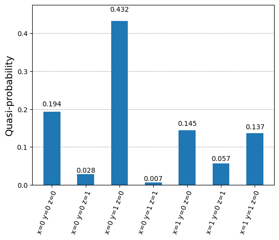
samples_for_plot = {
    " ".join(f"{qaoa_result.variables[i].name}={int(v)}" for i, v in enumerate(s.x)): s.probability
    for s in filtered_samples
}
samples_for_plot
[17]:
{'x=0 y=1 z=0': 0.4580078125,
 'x=0 y=0 z=0': 0.2255859375,
 'x=1 y=1 z=0': 0.12109375,
 'x=1 y=0 z=0': 0.1044921875,
 'x=1 y=0 z=1': 0.029296875,
 'x=0 y=1 z=1': 0.03515625,
 'x=0 y=0 z=1': 0.0244140625}
[18]:
plot_histogram(samples_for_plot)
[18]:
RecursiveMinimumEigenOptimizer
The RecursiveMinimumEigenOptimizer takes a MinimumEigenOptimizer as input and applies the recursive optimization scheme to reduce the size of the problem one variable at a time. Once the size of the generated intermediate problem is below a given threshold (min_num_vars), the RecursiveMinimumEigenOptimizer uses another solver (min_num_vars_optimizer), e.g., an exact classical solver such as CPLEX or the MinimumEigenOptimizer based on the NumPyMinimumEigensolver.
In the following, we show how to use the RecursiveMinimumEigenOptimizer using the two MinimumEigenOptimizers introduced before.
First, we construct the RecursiveMinimumEigenOptimizer such that it reduces the problem size from 3 variables to 1 variable and then uses the exact solver for the last variable. Then we call solve to optimize the considered problem.
[19]:
rqaoa = RecursiveMinimumEigenOptimizer(qaoa, min_num_vars=1, min_num_vars_optimizer=exact)
[20]:
rqaoa_result = rqaoa.solve(qubo)
print(rqaoa_result.prettyprint())
/Users/caw/Documents/GitHub/qiskit-braket-provider/qiskit_braket_provider/providers/adapter.py:860: UserWarning: The Qiskit circuit contains barrier instructions that are ignored.
  warnings.warn("The Qiskit circuit contains barrier instructions that are ignored.")
objective function value: -2.0
variable values: x=0.0, y=1.0, z=0.0
status: SUCCESS
[21]:
filtered_samples = get_filtered_samples(
    rqaoa_result.samples,
    threshold=0.005,
    allowed_status=(OptimizationResultStatus.SUCCESS,),
)
[22]:
samples_for_plot = {
    " ".join(f"{rqaoa_result.variables[i].name}={int(v)}" for i, v in enumerate(s.x)): s.probability
    for s in filtered_samples
}
samples_for_plot
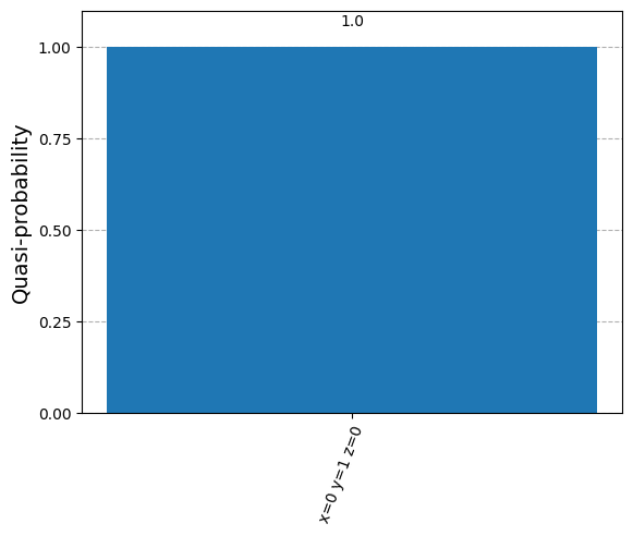
[22]:
{'x=0 y=1 z=0': 1.0}
[23]:
plot_histogram(samples_for_plot)
[23]: