Quantum Ensemble Learning Tutorial

Overview

This notebook demonstrates quantum ensemble learning for classification tasks using quantum cosine similarity classifiers. The approach combines multiple quantum classifiers through superposition to improve prediction accuracy and robustness.

Key Concepts

1. Quantum Cosine Classifier: Measures similarity between quantum-encoded data points

2. Quantum Ensemble: Creates superpositions of different training data arrangements

3. Random Unitary Ensemble: Uses randomly sampled unitaries for more general transformations

References

• This work: https://doi.org/10.1093/bib/bbag280

• Original ensemble work: Macaluso et al. IET Quantum Communication

• Original Code repository: GitHub

1. Setup and Initialization

%load_ext autoreload
%autoreload 2

import os
import numpy as np
import pandas as pd
import pickle
from collections import Counter
from sklearn import datasets
# Note: QBioCode also provides generate_blobs_datasets() for batch generation
# from qbiocode.data_generation import generate_blobs_datasets
from sklearn.model_selection import train_test_split
from sklearn.preprocessing import StandardScaler

# Use QBioCode API
from qbiocode.learning import compute_qensemble
from qbiocode.utils import (
    normalize_data,
    label_to_array,
    prepare_training_set,
    retrieve_probabilities
)
# Import helper functions for classical baselines and quantum workflows
from helper_functions import (
    evaluation_metrics,
    needs_run,
    run_random_forest,
    run_xgboost,
    run_lazy_predict,
    run_quantum_cosine,
    run_quantum_ensemble,
    post_process_results
)

<env>/lib/python3.12/site-packages/tqdm/auto.py:21: TqdmWarning: IProgress not found. Please update jupyter and ipywidgets. See https://ipywidgets.readthedocs.io/en/stable/user_install.html
  from .autonotebook import tqdm as notebook_tqdm

# Set random seed for reproducibility
seed = 54321
n_shots = 8192
np.random.seed(seed)

# Setup directories
DIR_HOME = '.'
DIR_OUTPUT = os.path.join(DIR_HOME, 'experiments')
os.makedirs(DIR_OUTPUT, exist_ok=True)

FILE_PREDICTIONS = os.path.join(DIR_OUTPUT, 'predictions.pkl')
FILE_DATASETS = os.path.join(DIR_OUTPUT, 'datasets.pkl')

2. Configuration Parameters

Define experiment parameters:

• TEST_SIZE: Fraction of data used for testing (0.2 = 20%)

• N_SPLITS: Number of cross-validation splits

• seed: Random seed for reproducibility

• n_shots: Number of quantum measurements per circuit

TEST_SIZE = 0.2
N_SPLITS = 5

# Load or initialize storage objects
if os.path.exists(FILE_DATASETS):
    dataset = pickle.load(open(FILE_DATASETS, 'rb'))
else:
    dataset = {}

if os.path.exists(FILE_PREDICTIONS):
    predictions = pickle.load(open(FILE_PREDICTIONS, 'rb'))
else:
    predictions = {}

3. Dataset Generation

Generate synthetic blob datasets with:

• 2D feature space: Easy to visualize

• 2 classes: Binary classification problem

• Varying parameters: Different cluster centers, standard deviations, and sample sizes

dataset_name = 'blob'
rerun = False
dataset_sizes = [20]

if (rerun) or (dataset_name not in dataset.keys()):
    predictions[dataset_name] = {}
    dataset[dataset_name] = {}

    for n_size in dataset_sizes:
        for std in [0.3, 0.5]:
            for p1 in [0.3, 0.5, 1]:
                for p2 in [0.3, 0.5, 1]:
                    centers = [[p1, p2], [p2, p1]]

                    for split in range(N_SPLITS):
                        X, y = datasets.make_blobs(
                            n_samples=n_size,
                            centers=centers,
                            n_features=2,
                            center_box=(0, 1),
                            cluster_std=std,
                            random_state=seed
                        )

                        X_train, X_test, y_train, y_test = train_test_split(
                            X, y, stratify=y, random_state=seed, test_size=TEST_SIZE
                        )

                        dataset[dataset_name][(split, n_size, std, p1, p2)] = (
                            pd.DataFrame(X_train),
                            pd.DataFrame(X_test),
                            pd.Series(y_train),
                            pd.Series(y_test)
                        )

    pickle.dump(dataset, open(FILE_DATASETS, 'wb'))

4. Classical Baselines

Run classical machine learning baselines for comparison.

Random Forest with Grid Search

method = 'random_forest_gs'
dataset_name = 'blob'
rerun = False

if needs_run(predictions, dataset_name, method, rerun):
    if dataset_name not in predictions.keys():
        predictions[dataset_name] = {}
    predictions = run_random_forest(predictions, dataset, method, dataset_name, seed, TEST_SIZE, FILE_PREDICTIONS)

Random Forest with Best Parameters

method = 'random_forest'
dataset_name = 'blob'
rerun = False

# Check if grid search results exist and have data
if 'random_forest_gs' in predictions.get(dataset_name, {}):
    # Select best parameters from grid search
    preds = predictions[dataset_name]['random_forest_gs']
    if len(preds) > 0 and 'best_params' in preds.columns:
        try:
            params_list = list(preds['best_params'])
            if len(params_list) > 0 and any(pd.notna(params_list)):
                params_map = dict(zip([str(x) for x in params_list], params_list))
                best = dict(Counter([str(x) for x in params_list]))
                if len(best) > 0:
                    best = pd.DataFrame([best.keys(), best.values()], index=['param', 'cnt']).transpose()
                    params = params_map[best[best.cnt == max(best.cnt)]['param'].iloc[0]]

                    if needs_run(predictions, dataset_name, method, rerun):
                        if dataset_name not in predictions.keys():
                            predictions[dataset_name] = {}
                        predictions = run_random_forest(predictions, dataset, method, dataset_name, seed, TEST_SIZE, FILE_PREDICTIONS, params=params)
                else:
                    print("No valid parameters found in grid search results. Skipping RF with best parameters.")
            else:
                print("Grid search parameters list is empty or contains only NaN values. Skipping RF with best parameters.")
        except Exception as e:
            print(f"Error processing grid search results: {e}. Skipping RF with best parameters.")
    else:
        print("Random Forest grid search results are empty or missing 'best_params' column. Skipping RF with best parameters.")
else:
    print("Random Forest grid search not run. Skipping RF with best parameters.")

XGBoost with Grid Search

method = 'xgb_gs'
dataset_name = 'blob'
rerun = False

if needs_run(predictions, dataset_name, method, rerun):
    if dataset_name not in predictions.keys():
        predictions[dataset_name] = {}
    predictions = run_xgboost(predictions, dataset, method, dataset_name, seed, TEST_SIZE, FILE_PREDICTIONS)

Fitting 3 folds for each of 486 candidates, totalling 1458 fits

XGBoost with Best Parameters

method = 'xgb'
dataset_name = 'blob'
rerun = False

# Import XGB_AVAILABLE flag from helper_functions
from helper_functions import XGB_AVAILABLE

# Check if XGBoost is installed and grid search results exist
if XGB_AVAILABLE and 'xgb_gs' in predictions.get(dataset_name, {}):
    # Select best parameters from grid search
    preds = predictions[dataset_name]['xgb_gs']
    if len(preds) > 0 and 'best_params' in preds.columns:
        try:
            params_list = list(preds['best_params'])
            if len(params_list) > 0 and any(pd.notna(params_list)):
                params_map = dict(zip([str(x) for x in params_list], params_list))
                best = dict(Counter([str(x) for x in params_list]))
                if len(best) > 0:
                    best = pd.DataFrame([best.keys(), best.values()], index=['param', 'cnt']).transpose()
                    params = params_map[best[best.cnt == max(best.cnt)]['param'].iloc[0]]

                    if needs_run(predictions, dataset_name, method, rerun):
                        if dataset_name not in predictions.keys():
                            predictions[dataset_name] = {}
                        predictions = run_xgboost(predictions, dataset, method, dataset_name, seed, TEST_SIZE, FILE_PREDICTIONS, params=params)
                else:
                    print("No valid parameters found in XGBoost grid search results. Skipping XGBoost with best parameters.")
            else:
                print("XGBoost grid search parameters list is empty or contains only NaN values. Skipping XGBoost with best parameters.")
        except Exception as e:
            print(f"Error processing XGBoost grid search results: {e}. Skipping XGBoost with best parameters.")
    else:
        print("XGBoost grid search results are empty or missing 'best_params' column. Skipping XGBoost with best parameters.")
else:
    if not XGB_AVAILABLE:
        print('XGBoost not installed. Install with: pip install xgboost')
        print('Note: On macOS, you may also need to install libomp: brew install libomp')
    else:
        print('XGBoost grid search not run. Skipping XGBoost with best parameters.')

5. Quantum Cosine Classifier

The quantum cosine classifier measures similarity between quantum states using:

1. State Preparation: Encode classical data as quantum states

2. Controlled-SWAP Test: Measure overlap between training and test states

3. Hadamard Interference: Extract similarity information

4. Measurement: Obtain classification probability

Key Parameters:

• n_train: Number of training samples (typically 1 for single classifier)

• n_features: Number of features (must be power of 2)

• n_shots: Measurement shots for probability estimation

method = 'qcosine'
rerun = False
n_trains = [1]
n_features = [2]

if needs_run(predictions, dataset_name, method, rerun):
    predictions = run_quantum_cosine(
        predictions, dataset, method, dataset_name, seed, TEST_SIZE, FILE_PREDICTIONS,
        n_features, n_trains, n_shots
    )

6. Quantum Ensemble Method

The quantum ensemble creates superpositions of different training data arrangements using controlled swap operations.

Algorithm:

1. Initialize control qubits in superposition (Hadamard gates)

2. Apply controlled swaps to rearrange training data

3. Perform cosine similarity test

4. Measure to obtain ensemble prediction

Key Parameters:

• d: Number of control qubits (ensemble depth) - creates 2^d ensemble members

• n_swap: Number of swap operations per control qubit

• n_train: Number of training samples (must be even for balanced mode)

• mode: Sampling strategy (“balanced”, “unbalanced”, “pair_sample”)

method = 'qensemble'
rerun = False
ds = [1, 2]
n_trains = [2, 4]
n_swaps = [1, 2]
n_features = [2]
pca_embed = False
umap_embed = False
device = 'CPU'

if needs_run(predictions, dataset_name, method, rerun):
    predictions = run_quantum_ensemble(
        predictions, dataset, method, dataset_name, seed, TEST_SIZE, FILE_PREDICTIONS,
        ds, n_swaps, n_features, n_trains, n_shots,
        pca_embed=pca_embed, umap_embed=umap_embed, device=device
    )

7. Random Unitary Ensemble

This advanced variant uses randomly sampled unitaries instead of fixed swap patterns.

Advantages:

• More general transformations of training data

• Potentially better exploration of hypothesis space

• Theoretical connections to quantum advantage

Trade-offs:

• Higher circuit depth and complexity

• More difficult to implement on real quantum hardware

• Potentially better generalization

Note: This method is more computationally intensive but may provide better results on complex datasets.

method = 'qensemble_random_unitary'
rerun = False
ds = [1]
n_trains = [2]
n_swaps = [1]
n_features = [2]
pca_embed = False
umap_embed = False
device = 'CPU'

if needs_run(predictions, dataset_name, method, rerun):
    predictions = run_quantum_ensemble(
        predictions, dataset, method, dataset_name, seed, TEST_SIZE, FILE_PREDICTIONS,
        ds, n_swaps, n_features, n_trains, n_shots,
        pca_embed=pca_embed, umap_embed=umap_embed, device=device,
        random_unitary=True
    )

8. Results Visualization

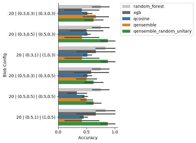
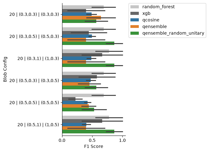
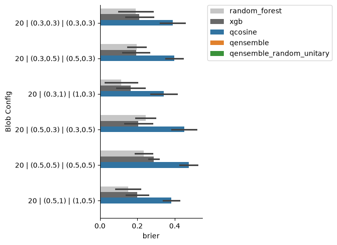
Process and visualize the results from all methods. Per Blob configuration, plot the best performing method configuration (maximum median metric score). Saves the full statistics to a CSV file at experiments/Blobs_best_stats.csv

# Post-process results
total_results_full, sig_bestmethods_df = post_process_results(predictions, DIR_OUTPUT, datasets=['blob'])

Dataset: blob
Method: random_forest
Method: qcosine
Method: qensemble
Method: qensemble_random_unitary
Method: xgb
XGB: blob : random_forest (n=90) : t=4.87; p=0.0
XGB: blob : qensemble (n=90) : t=1.975; p=0.025
XGB: blob : qensemble_random_unitary (n=90) : t=5.42; p=0.0

XGB: blob : random_forest (n=90) : t=3.977; p=0.0
XGB: blob : qensemble (n=90) : t=2.039; p=0.021
XGB: blob : qensemble_random_unitary (n=90) : t=5.187; p=0.0

Conclusion

This tutorial demonstrated quantum ensemble learning for classification:

Key Takeaways

1. Quantum Ensembling: Ensemble methods leverage quantum superposition to evaluate multiple classifiers simultaneously

2. Parameter Tuning: Performance depends on careful selection of d, n_swap, and n_train

3. Trade-offs: Balance between accuracy improvement and computational cost

4. Scalability: Current methods limited by qubit count (~30-36 for simulation)

Next Steps

• Test on real quantum hardware (IBM Quantum, etc.)

• Apply to real-world datasets

• Explore error mitigation techniques

• Investigate theoretical quantum advantage

Further Reading

• See README.md for detailed documentation

• Refer to cited papers for theoretical background