Quantum State Tomography
Quantum tomography is an experimental procedure to reconstruct a description of part of a quantum system from the measurement outcomes of a specific set of experiments. In particular, quantum state tomography reconstructs the density matrix of a quantum state by preparing the state many times and measuring them in a tomographically complete basis of measurement operators.
Note
This tutorial requires the qiskit-aer and qiskit-ibm-runtime
packages to run simulations. You can install them with python -m pip
install qiskit-aer qiskit-ibm-runtime.
We first initialize a simulator to run the experiments on.
from qiskit_aer import AerSimulator
from qiskit_ibm_runtime.fake_provider import FakePerth

backend = AerSimulator.from_backend(FakePerth())
To run a state tomography experiment, we initialize the experiment with a circuit to
prepare the state to be measured. We can also pass in an
Operator or a Statevector
to describe the preparation circuit.
import qiskit
from qiskit_experiments.framework import ParallelExperiment
from qiskit_experiments.library import StateTomography

# GHZ State preparation circuit
nq = 2
qc_ghz = qiskit.QuantumCircuit(nq)
qc_ghz.h(0)
qc_ghz.s(0)
for i in range(1, nq):
    qc_ghz.cx(0, i)

# QST Experiment
qstexp1 = StateTomography(qc_ghz)
qstdata1 = qstexp1.run(backend, seed_simulation=100).block_for_results()

# Print results
display(qstdata1.analysis_results(dataframe=True))
| name | experiment | components | value | quality | backend | run_time | trace | eigvals | raw_eigvals | rescaled_psd | fitter_metadata | conditional_probability | positive | |
|---|---|---|---|---|---|---|---|---|---|---|---|---|---|---|
| 972969c6 | state | StateTomography | [Q0, Q1] | DensityMatrix([[ 0.47135417+0.j , -0.00... | None | aer_simulator_from(fake_perth) | None | 1.0 | [0.9089995856027787, 0.044523537286277434, 0.0... | [0.9089995856027787, 0.044523537286277434, 0.0... | False | {'fitter': 'linear_inversion', 'fitter_time': ... | 1.0 | True |
| 3bffc9ea | state_fidelity | StateTomography | [Q0, Q1] | 0.908691 | None | aer_simulator_from(fake_perth) | None | None | None | None | None | None | None | None |
| 481f8019 | positive | StateTomography | [Q0, Q1] | True | None | aer_simulator_from(fake_perth) | None | None | None | None | None | None | None | None |
Tomography Results
The main result for tomography is the fitted state, which is stored as a
DensityMatrix object:
state_result = qstdata1.analysis_results("state", dataframe=True).iloc[0]
print(state_result.value)
DensityMatrix([[ 0.47135417+0.j        , -0.00569661+0.01123047j,
                -0.00830078+0.00878906j,  0.01123047-0.4375j    ],
               [-0.00569661-0.01123047j,  0.03320313+0.j        ,
                -0.00048828-0.00488281j, -0.00244141+0.00097656j],
               [-0.00830078-0.00878906j, -0.00048828+0.00488281j,
                 0.02441406+0.j        ,  0.00309245-0.00341797j],
               [ 0.01123047+0.4375j    , -0.00244141-0.00097656j,
                 0.00309245+0.00341797j,  0.47102865+0.j        ]],
              dims=(2, 2))
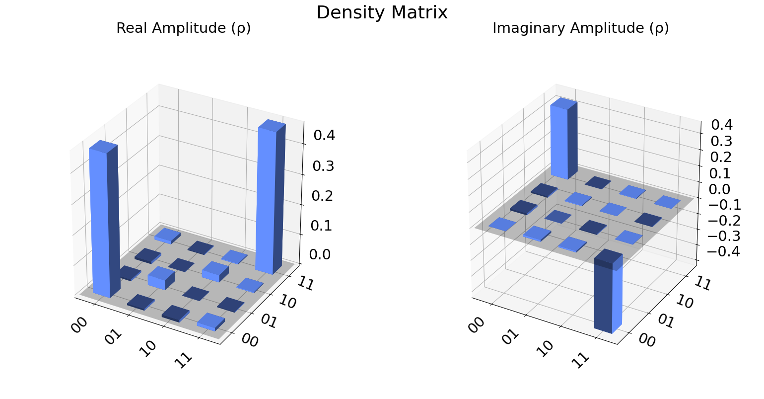
We can also visualize the density matrix:
from qiskit.visualization import plot_state_city
state = qstdata1.analysis_results("state", dataframe=True).iloc[0].value
plot_state_city(state, title='Density Matrix')
The state fidelity of the fitted state with the ideal state prepared by
the input circuit is stored in the "state_fidelity" result field.
Note that if the input circuit contained any measurements the ideal
state cannot be automatically generated and this field will be set to
None.
fid_result = qstdata1.analysis_results("state_fidelity", dataframe=True).iloc[0]
print("State Fidelity = {:.5f}".format(fid_result.value))
State Fidelity = 0.90869
Additional state metadata
Additional data is stored in the tomography under additional fields. This includes
eigvals: the eigenvalues of the fitted statetrace: the trace of the fitted statepositive: Whether the eigenvalues are all non-negative
If trace rescaling was performed this dictionary will also contain a raw_trace field
containing the trace before rescaling. Futhermore, if the state was rescaled to be
positive or trace 1 an additional field raw_eigvals will contain the state
eigenvalues before rescaling was performed.
for col in ["eigvals", "trace", "positive"]:
    print(f"{col}: {state_result[col]}")
eigvals: [0.90899959 0.04452354 0.03265294 0.01382394]
trace: 1.0000000000000018
positive: True
To see the effect of rescaling, we can perform a “bad” fit with very low counts:
# QST Experiment
bad_data = qstexp1.run(backend, shots=10, seed_simulation=100).block_for_results()
bad_state_result = bad_data.analysis_results("state", dataframe=True).iloc[0]

# Print result
for key, val in bad_state_result.items():
    print(f"{key}: {val}")
name: state
experiment: StateTomography
components: [<Qubit(Q0)>, <Qubit(Q1)>]
value: DensityMatrix([[ 0.43147144+0.00000000e+00j, -0.08330658+2.42649578e-02j,
                 0.02938817+3.91367053e-02j, -0.05044674-3.91895459e-01j],
               [-0.08330658-2.42649578e-02j,  0.0821308 -9.75781955e-19j,
                -0.0179613 +9.34165102e-03j,  0.0075933 +1.60644283e-01j],
               [ 0.02938817-3.91367053e-02j, -0.0179613 -9.34165102e-03j,
                 0.01411713+2.16840434e-19j, -0.01988044-4.62210223e-02j],
               [-0.05044674+3.91895459e-01j,  0.0075933 -1.60644283e-01j,
                -0.01988044+4.62210223e-02j,  0.47228064+0.00000000e+00j]],
              dims=(2, 2))
quality: None
backend: aer_simulator_from(fake_perth)
run_time: None
trace: 1.0000000000000009
eigvals: [0.89107219 0.10892781 0.         0.        ]
raw_eigvals: [ 1.00367009  0.2215257  -0.05299492 -0.17220088]
rescaled_psd: True
fitter_metadata: {'fitter': 'linear_inversion', 'fitter_time': 0.002903461456298828}
conditional_probability: 1.0
positive: True
Tomography Fitters
The default fitters is linear_inversion, which reconstructs the
state using dual basis of the tomography basis. This will typically
result in a non-positive reconstructed state. This state is rescaled to
be positive-semidefinite (PSD) by computing its eigen-decomposition and
rescaling its eigenvalues using the approach from Ref. [1].
There are several other fitters are included (See API documentation for
details). For example, if cvxpy is installed we can use the
cvxpy_gaussian_lstsq() fitter, which allows constraining the fit to be
PSD without requiring rescaling.
try:
    import cvxpy

    # Set analysis option for cvxpy fitter
    qstexp1.analysis.set_options(fitter='cvxpy_gaussian_lstsq')

    # Re-run experiment
    qstdata2 = qstexp1.run(backend, seed_simulation=100).block_for_results()

    state_result2 = qstdata2.analysis_results("state", dataframe=True).iloc[0]
    for key, val in state_result2.items():
        print(f"{key}: {val}")

except ModuleNotFoundError:
    print("CVXPY is not installed")
name: state
experiment: StateTomography
components: [<Qubit(Q0)>, <Qubit(Q1)>]
value: DensityMatrix([[ 0.48882957+0.j        , -0.00777928+0.01274733j,
                -0.00155392-0.00749651j, -0.00658826-0.44162226j],
               [-0.00777928-0.01274733j,  0.02440825+0.j        ,
                 0.01863236+0.00719646j, -0.00065324-0.00551869j],
               [-0.00155392+0.00749651j,  0.01863236-0.00719646j,
                 0.02738331+0.j        ,  0.01427616-0.01229179j],
               [-0.00658826+0.44162226j, -0.00065324+0.00551869j,
                 0.01427616+0.01229179j,  0.45937888+0.j        ]],
              dims=(2, 2))
quality: None
backend: aer_simulator_from(fake_perth)
run_time: None
trace: 1.0000000012913224
eigvals: [0.91644656 0.05707558 0.02118944 0.00528842]
raw_eigvals: [0.91644656 0.05707558 0.02118944 0.00528842]
rescaled_psd: False
fitter_metadata: {'fitter': 'cvxpy_gaussian_lstsq', 'cvxpy_solver': 'SCS', 'cvxpy_status': ['optimal'], 'psd_constraint': True, 'trace_preserving': True, 'fitter_time': 0.03039836883544922}
conditional_probability: 1.0
positive: True
Parallel Tomography Experiment
We can also use the ParallelExperiment class to
run subsystem tomography on multiple qubits in parallel.
For example if we want to perform 1-qubit QST on several qubits at once:
from math import pi
num_qubits = 5
gates = [qiskit.circuit.library.RXGate(i * pi / (num_qubits - 1))
         for i in range(num_qubits)]

subexps = [
    StateTomography(gate, physical_qubits=(i,))
    for i, gate in enumerate(gates)
]
parexp = ParallelExperiment(subexps)
pardata = parexp.run(backend, seed_simulation=100).block_for_results()

display(pardata.analysis_results(dataframe=True))
| name | experiment | components | value | quality | backend | run_time | trace | eigvals | raw_eigvals | rescaled_psd | fitter_metadata | conditional_probability | positive | |
|---|---|---|---|---|---|---|---|---|---|---|---|---|---|---|
| de37e53e | state | StateTomography | [Q0] | DensityMatrix([[ 0.96582031+0.j , -0.02... | None | aer_simulator_from(fake_perth) | None | 1.0 | [0.9664463658548947, 0.03355363414510623] | [0.9664463658548947, 0.03355363414510623] | False | {'fitter': 'linear_inversion', 'fitter_time': ... | 1.0 | True |
| 852dac49 | state_fidelity | StateTomography | [Q0] | 0.96582 | None | aer_simulator_from(fake_perth) | None | None | None | None | None | None | None | None |
| 4babeff8 | positive | StateTomography | [Q0] | True | None | aer_simulator_from(fake_perth) | None | None | None | None | None | None | None | None |
| b276d5ec | state | StateTomography | [Q1] | DensityMatrix([[ 0.83007813+0.j , -0.01... | None | aer_simulator_from(fake_perth) | None | 1.0 | [0.9731785434272788, 0.02682145657272214] | [0.9731785434272788, 0.02682145657272214] | False | {'fitter': 'linear_inversion', 'fitter_time': ... | 1.0 | True |
| df8fd64e | state_fidelity | StateTomography | [Q1] | 0.973016 | None | aer_simulator_from(fake_perth) | None | None | None | None | None | None | None | None |
| f35d314f | positive | StateTomography | [Q1] | True | None | aer_simulator_from(fake_perth) | None | None | None | None | None | None | None | None |
| 7d7df8cc | state | StateTomography | [Q2] | DensityMatrix([[0.4921875 +0.j , 0.0126... | None | aer_simulator_from(fake_perth) | None | 1.0 | [0.9621545274591357, 0.03784547254086543] | [0.9621545274591357, 0.03784547254086543] | False | {'fitter': 'linear_inversion', 'fitter_time': ... | 1.0 | True |
| bd624eb3 | state_fidelity | StateTomography | [Q2] | 0.961914 | None | aer_simulator_from(fake_perth) | None | None | None | None | None | None | None | None |
| 319dfdcf | positive | StateTomography | [Q2] | True | None | aer_simulator_from(fake_perth) | None | None | None | None | None | None | None | None |
| b4f08315 | state | StateTomography | [Q3] | DensityMatrix([[0.16210938+0.j , 0.0263... | None | aer_simulator_from(fake_perth) | None | 1.0 | [0.9724120462895633, 0.02758795371043772] | [0.9724120462895633, 0.02758795371043772] | False | {'fitter': 'linear_inversion', 'fitter_time': ... | 1.0 | True |
| 7c7a4e27 | state_fidelity | StateTomography | [Q3] | 0.971635 | None | aer_simulator_from(fake_perth) | None | None | None | None | None | None | None | None |
| 700bc9fb | positive | StateTomography | [Q3] | True | None | aer_simulator_from(fake_perth) | None | None | None | None | None | None | None | None |
| 03a96995 | state | StateTomography | [Q4] | DensityMatrix([[0.03027344+0.j , 0.0097... | None | aer_simulator_from(fake_perth) | None | 1.0 | [0.9703190292969741, 0.029680970703027193] | [0.9703190292969741, 0.029680970703027193] | False | {'fitter': 'linear_inversion', 'fitter_time': ... | 1.0 | True |
| 2bece033 | state_fidelity | StateTomography | [Q4] | 0.969727 | None | aer_simulator_from(fake_perth) | None | None | None | None | None | None | None | None |
| 9ed8f1ed | positive | StateTomography | [Q4] | True | None | aer_simulator_from(fake_perth) | None | None | None | None | None | None | None | None |
View experiment analysis results for one component:
results = pardata.analysis_results(dataframe=True)
display(results[results.components.apply(lambda x: x == ["Q0"])])
| name | experiment | components | value | quality | backend | run_time | trace | eigvals | raw_eigvals | rescaled_psd | fitter_metadata | conditional_probability | positive | |
|---|---|---|---|---|---|---|---|---|---|---|---|---|---|---|
| de37e53e | state | StateTomography | [Q0] | DensityMatrix([[ 0.96582031+0.j , -0.02... | None | aer_simulator_from(fake_perth) | None | 1.0 | [0.9664463658548947, 0.03355363414510623] | [0.9664463658548947, 0.03355363414510623] | False | {'fitter': 'linear_inversion', 'fitter_time': ... | 1.0 | True |
| 852dac49 | state_fidelity | StateTomography | [Q0] | 0.96582 | None | aer_simulator_from(fake_perth) | None | None | None | None | None | None | None | None |
| 4babeff8 | positive | StateTomography | [Q0] | True | None | aer_simulator_from(fake_perth) | None | None | None | None | None | None | None | None |
References
See also
API documentation:
StateTomography