Quantum State Tomography

Quantum tomography is an experimental procedure to reconstruct a description of part of a quantum system from the measurement outcomes of a specific set of experiments. In particular, quantum state tomography reconstructs the density matrix of a quantum state by preparing the state many times and measuring them in a tomographically complete basis of measurement operators.

Note

This tutorial requires the qiskit-aer and qiskit-ibm-runtime packages to run simulations. You can install them with python -m pip install qiskit-aer qiskit-ibm-runtime.

We first initialize a simulator to run the experiments on.

from qiskit_aer import AerSimulator
from qiskit_ibm_runtime.fake_provider import FakePerth

backend = AerSimulator.from_backend(FakePerth())

To run a state tomography experiment, we initialize the experiment with a circuit to prepare the state to be measured. We can also pass in an Operator or a Statevector to describe the preparation circuit.

import qiskit
from qiskit_experiments.framework import ParallelExperiment
from qiskit_experiments.library import StateTomography

# GHZ State preparation circuit
nq = 2
qc_ghz = qiskit.QuantumCircuit(nq)
qc_ghz.h(0)
qc_ghz.s(0)
for i in range(1, nq):
    qc_ghz.cx(0, i)

# QST Experiment
qstexp1 = StateTomography(qc_ghz)
qstdata1 = qstexp1.run(backend, seed_simulation=100).block_for_results()

# Print results
for result in qstdata1.analysis_results():
    print(result)

AnalysisResult
- name: state
- value: DensityMatrix([[ 0.47607422+0.j        ,  0.01057943-0.00211589j,
                -0.00878906+0.01855469j,  0.00732422-0.453125j  ],
               [ 0.01057943+0.00211589j,  0.02457682+0.j        ,
                 0.01123047-0.00195312j,  0.00585938-0.01757812j],
               [-0.00878906-0.01855469j,  0.01123047+0.00195312j,
                 0.02620443+0.j        , -0.00309245-0.00211589j],
               [ 0.00732422+0.453125j  ,  0.00585938+0.01757812j,
                -0.00309245+0.00211589j,  0.47314453+0.j        ]],
              dims=(2, 2))
- quality: unknown
- extra: <9 items>
- device_components: ['Q0', 'Q1']
- verified: False
AnalysisResult
- name: state_fidelity
- value: 0.9277343749999996
- quality: unknown
- extra: <9 items>
- device_components: ['Q0', 'Q1']
- verified: False
AnalysisResult
- name: positive
- value: True
- quality: unknown
- extra: <9 items>
- device_components: ['Q0', 'Q1']
- verified: False

Tomography Results

The main result for tomography is the fitted state, which is stored as a DensityMatrix object:

state_result = qstdata1.analysis_results("state")
print(state_result.value)

DensityMatrix([[ 0.47607422+0.j        ,  0.01057943-0.00211589j,
                -0.00878906+0.01855469j,  0.00732422-0.453125j  ],
               [ 0.01057943+0.00211589j,  0.02457682+0.j        ,
                 0.01123047-0.00195312j,  0.00585938-0.01757812j],
               [-0.00878906-0.01855469j,  0.01123047+0.00195312j,
                 0.02620443+0.j        , -0.00309245-0.00211589j],
               [ 0.00732422+0.453125j  ,  0.00585938+0.01757812j,
                -0.00309245+0.00211589j,  0.47314453+0.j        ]],
              dims=(2, 2))

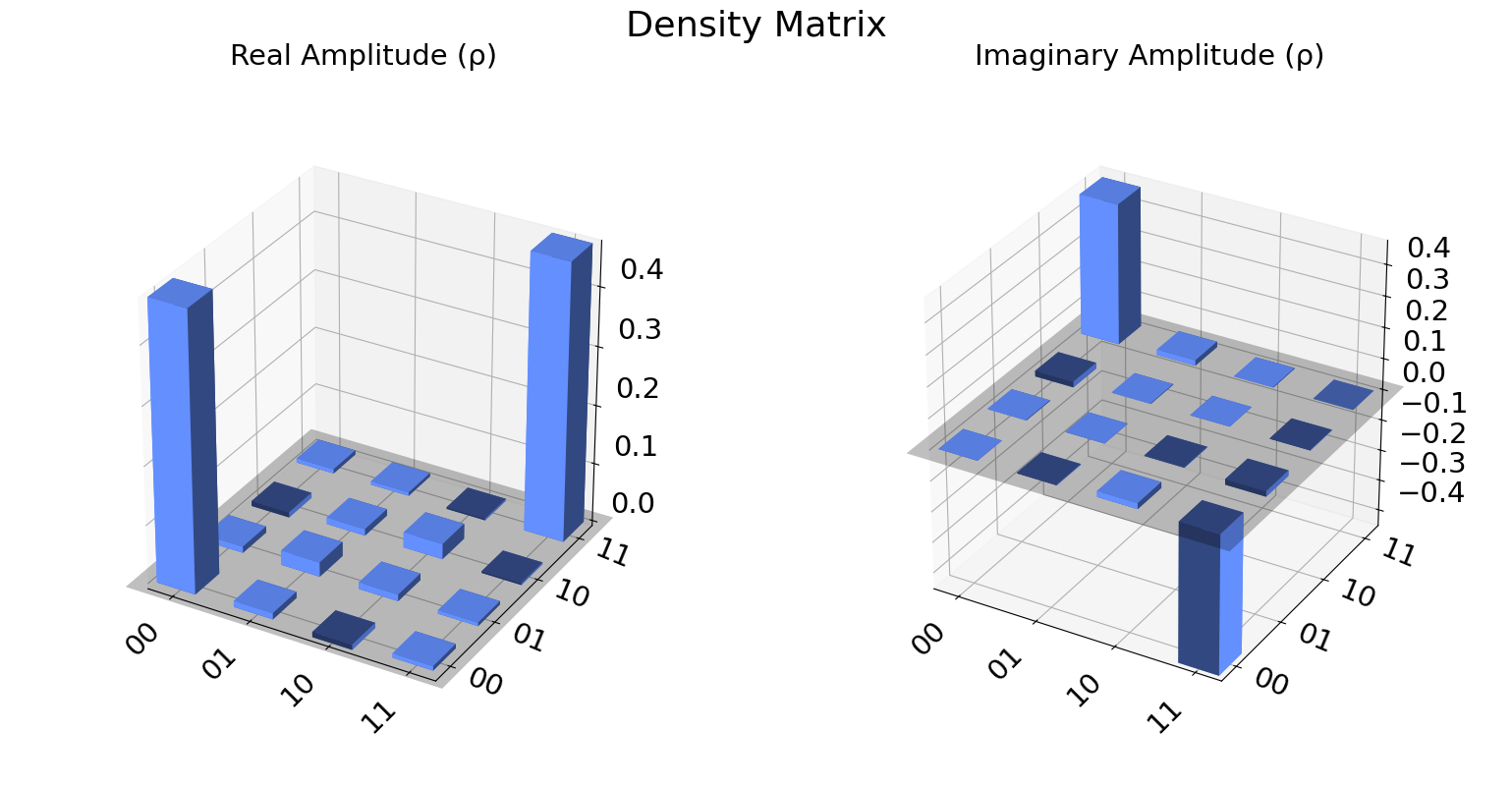
We can also visualize the density matrix:

from qiskit.visualization import plot_state_city
plot_state_city(qstdata1.analysis_results("state").value, title='Density Matrix')

The state fidelity of the fitted state with the ideal state prepared by the input circuit is stored in the "state_fidelity" result field. Note that if the input circuit contained any measurements the ideal state cannot be automatically generated and this field will be set to None.

fid_result = qstdata1.analysis_results("state_fidelity")
print("State Fidelity = {:.5f}".format(fid_result.value))

State Fidelity = 0.92773

Additional state metadata

Additional data is stored in the tomography under the "state_metadata" field. This includes

• eigvals: the eigenvalues of the fitted state

• trace: the trace of the fitted state

• positive: Whether the eigenvalues are all non-negative

• positive_delta: the deviation from positivity given by 1-norm of negative eigenvalues.

If trace rescaling was performed this dictionary will also contain a raw_trace field containing the trace before rescaling. Futhermore, if the state was rescaled to be positive or trace 1 an additional field raw_eigvals will contain the state eigenvalues before rescaling was performed.

state_result.extra

{'trace': 1.0000000000000018,
 'eigvals': array([0.92854978, 0.04475651, 0.01788861, 0.00880509]),
 'raw_eigvals': array([0.92854978, 0.04475651, 0.01788861, 0.00880509]),
 'rescaled_psd': False,
 'fitter_metadata': {'fitter': 'linear_inversion',
  'fitter_time': 0.0081634521484375},
 'conditional_probability': 1.0,
 'positive': True,
 'experiment': 'StateTomography',
 'run_time': None}

To see the effect of rescaling, we can perform a “bad” fit with very low counts:

# QST Experiment
bad_data = qstexp1.run(backend, shots=10, seed_simulation=100).block_for_results()
bad_state_result = bad_data.analysis_results("state")

# Print result
print(bad_state_result)

# Show extra data
bad_state_result.extra

AnalysisResult
- name: state
- value: DensityMatrix([[ 0.47217108+0.00000000e+00j,  0.02909732-1.04242807e-01j,
                 0.0426279 +7.42622568e-02j, -0.13266668-4.18813520e-01j],
               [ 0.02909732+1.04242807e-01j,  0.06213807+1.11130723e-18j,
                -0.02567935+2.37324645e-02j,  0.0494422 -4.53760420e-02j],
               [ 0.0426279 -7.42622568e-02j, -0.02567935-2.37324645e-02j,
                 0.02187265+1.73472348e-18j, -0.06419152-1.09511942e-02j],
               [-0.13266668+4.18813520e-01j,  0.0494422 +4.53760420e-02j,
                -0.06419152+1.09511942e-02j,  0.4438182 -2.77555756e-17j]],
              dims=(2, 2))
- quality: unknown
- extra: <9 items>
- device_components: ['Q0', 'Q1']
- verified: False

{'trace': 1.0000000000000007,
 'eigvals': array([0.92912346, 0.07087654, 0.        , 0.        ]),
 'raw_eigvals': array([ 1.00551049,  0.14726357,  0.02370439, -0.17647845]),
 'rescaled_psd': True,
 'fitter_metadata': {'fitter': 'linear_inversion',
  'fitter_time': 0.0050106048583984375},
 'conditional_probability': 1.0,
 'positive': True,
 'experiment': 'StateTomography',
 'run_time': None}

Tomography Fitters

The default fitters is linear_inversion, which reconstructs the state using dual basis of the tomography basis. This will typically result in a non-positive reconstructed state. This state is rescaled to be positive-semidefinite (PSD) by computing its eigen-decomposition and rescaling its eigenvalues using the approach from Ref. [1].

There are several other fitters are included (See API documentation for details). For example, if cvxpy is installed we can use the cvxpy_gaussian_lstsq() fitter, which allows constraining the fit to be PSD without requiring rescaling.

try:
    import cvxpy

    # Set analysis option for cvxpy fitter
    qstexp1.analysis.set_options(fitter='cvxpy_gaussian_lstsq')

    # Re-run experiment
    qstdata2 = qstexp1.run(backend, seed_simulation=100).block_for_results()

    state_result2 = qstdata2.analysis_results("state")
    print(state_result2)
    print("\nextra:")
    for key, val in state_result2.extra.items():
        print(f"- {key}: {val}")

except ModuleNotFoundError:
    print("CVXPY is not installed")

AnalysisResult
- name: state
- value: DensityMatrix([[ 4.87689601e-01+0.j        ,  2.11762284e-04-0.00351974j,
                 2.02147837e-02-0.01013156j,  3.54292357e-03-0.44953316j],
               [ 2.11762284e-04+0.00351974j,  2.06187964e-02+0.j        ,
                 1.38352871e-02-0.0016599j , -1.08834592e-02+0.02251748j],
               [ 2.02147837e-02+0.01013156j,  1.38352871e-02+0.0016599j ,
                 1.49130222e-02+0.j        , -1.30427056e-02-0.00551499j],
               [ 3.54292357e-03+0.44953316j, -1.08834592e-02-0.02251748j,
                -1.30427056e-02+0.00551499j,  4.76778581e-01+0.j        ]],
              dims=(2, 2))
- quality: unknown
- extra: <9 items>
- device_components: ['Q0', 'Q1']
- verified: False

extra:
- trace: 0.9999999992602469
- eigvals: [9.32469754e-01 5.92595004e-02 8.24585221e-03 2.48936350e-05]
- raw_eigvals: [9.32469754e-01 5.92595004e-02 8.24585222e-03 2.48936350e-05]
- rescaled_psd: False
- fitter_metadata: {'fitter': 'cvxpy_gaussian_lstsq', 'cvxpy_solver': 'SCS', 'cvxpy_status': ['optimal'], 'psd_constraint': True, 'trace_preserving': True, 'fitter_time': 0.021259784698486328}
- conditional_probability: 1.0
- positive: True
- experiment: StateTomography
- run_time: None

Parallel Tomography Experiment

We can also use the ParallelExperiment class to run subsystem tomography on multiple qubits in parallel.

For example if we want to perform 1-qubit QST on several qubits at once:

from math import pi
num_qubits = 5
gates = [qiskit.circuit.library.RXGate(i * pi / (num_qubits - 1))
         for i in range(num_qubits)]

subexps = [
    StateTomography(gate, physical_qubits=(i,))
    for i, gate in enumerate(gates)
]
parexp = ParallelExperiment(subexps)
pardata = parexp.run(backend, seed_simulation=100).block_for_results()

for result in pardata.analysis_results():
    print(result)

AnalysisResult
- name: state
- value: DensityMatrix([[0.97460938+0.j        , 0.015625  +0.00683594j],
               [0.015625  -0.00683594j, 0.02539063+0.j        ]],
              dims=(2,))
- quality: unknown
- extra: <9 items>
- device_components: ['Q0']
- verified: False
AnalysisResult
- name: state_fidelity
- value: 0.974609375
- quality: unknown
- extra: <9 items>
- device_components: ['Q0']
- verified: False
AnalysisResult
- name: positive
- value: True
- quality: unknown
- extra: <9 items>
- device_components: ['Q0']
- verified: False
AnalysisResult
- name: state
- value: DensityMatrix([[ 0.83007813+0.j        , -0.00292969+0.35546875j],
               [-0.00292969-0.35546875j,  0.16992188+0.j        ]],
              dims=(2,))
- quality: unknown
- extra: <9 items>
- device_components: ['Q1']
- verified: False
AnalysisResult
- name: state_fidelity
- value: 0.9847548441337468
- quality: unknown
- extra: <9 items>
- device_components: ['Q1']
- verified: False
AnalysisResult
- name: positive
- value: True
- quality: unknown
- extra: <9 items>
- device_components: ['Q1']
- verified: False
AnalysisResult
- name: state
- value: DensityMatrix([[ 0.51367188+0.j        , -0.00195312+0.47949219j],
               [-0.00195312-0.47949219j,  0.48632813+0.j        ]],
              dims=(2,))
- quality: unknown
- extra: <9 items>
- device_components: ['Q2']
- verified: False
AnalysisResult
- name: state_fidelity
- value: 0.9794921875000004
- quality: unknown
- extra: <9 items>
- device_components: ['Q2']
- verified: False
AnalysisResult
- name: positive
- value: True
- quality: unknown
- extra: <9 items>
- device_components: ['Q2']
- verified: False
AnalysisResult
- name: state
- value: DensityMatrix([[0.17285156+0.j        , 0.01757812+0.33886719j],
               [0.01757812-0.33886719j, 0.82714844+0.j        ]],
              dims=(2,))
- quality: unknown
- extra: <9 items>
- device_components: ['Q3']
- verified: False
AnalysisResult
- name: state_fidelity
- value: 0.9709441648136968
- quality: unknown
- extra: <9 items>
- device_components: ['Q3']
- verified: False
AnalysisResult
- name: positive
- value: True
- quality: unknown
- extra: <9 items>
- device_components: ['Q3']
- verified: False
AnalysisResult
- name: state
- value: DensityMatrix([[ 0.03417969+0.j        , -0.015625  -0.00683594j],
               [-0.015625  +0.00683594j,  0.96582031+0.j        ]],
              dims=(2,))
- quality: unknown
- extra: <9 items>
- device_components: ['Q4']
- verified: False
AnalysisResult
- name: state_fidelity
- value: 0.9658203125000006
- quality: unknown
- extra: <9 items>
- device_components: ['Q4']
- verified: False
AnalysisResult
- name: positive
- value: True
- quality: unknown
- extra: <9 items>
- device_components: ['Q4']
- verified: False

View component experiment analysis results:

for i, expdata in enumerate(pardata.child_data()):
    state_result_i = expdata.analysis_results("state")
    fid_result_i = expdata.analysis_results("state_fidelity")

    print(f'\nPARALLEL EXP {i}')
    print("State Fidelity: {:.5f}".format(fid_result_i.value))
    print("State: {}".format(state_result_i.value))

References

[1]

J Smolin, JM Gambetta, G Smith, Phys. Rev. Lett. 108, 070502 (2012), open access.

See also

• API documentation: StateTomography