Quantum State Tomography
Quantum tomography is an experimental procedure to reconstruct a description of part of a quantum system from the measurement outcomes of a specific set of experiments. In particular, quantum state tomography reconstructs the density matrix of a quantum state by preparing the state many times and measuring them in a tomographically complete basis of measurement operators.
Note
This tutorial requires the qiskit-aer and qiskit-ibm-runtime
packages to run simulations. You can install them with python -m pip
install qiskit-aer qiskit-ibm-runtime.
We first initialize a simulator to run the experiments on.
from qiskit_aer import AerSimulator
from qiskit_ibm_runtime.fake_provider import FakePerth

backend = AerSimulator.from_backend(FakePerth())
To run a state tomography experiment, we initialize the experiment with a circuit to
prepare the state to be measured. We can also pass in an
Operator or a Statevector
to describe the preparation circuit.
import qiskit
from qiskit_experiments.framework import ParallelExperiment
from qiskit_experiments.library import StateTomography

# GHZ State preparation circuit
nq = 2
qc_ghz = qiskit.QuantumCircuit(nq)
qc_ghz.h(0)
qc_ghz.s(0)
for i in range(1, nq):
    qc_ghz.cx(0, i)

# QST Experiment
qstexp1 = StateTomography(qc_ghz)
qstdata1 = qstexp1.run(backend, seed_simulation=100).block_for_results()

# Print results
for result in qstdata1.analysis_results():
    print(result)
AnalysisResult
- name: state
- value: DensityMatrix([[ 0.48140875+0.00000000e+00j,  0.01000945+2.04374247e-03j,
                -0.00791127-6.61105019e-03j,  0.0117096 -4.52705410e-01j],
               [ 0.01000945-2.04374247e-03j,  0.01193548-4.33680869e-19j,
                -0.00621776+3.47478180e-03j, -0.00363127+9.83180696e-03j],
               [-0.00791127+6.61105019e-03j, -0.00621776-3.47478180e-03j,
                 0.03076499+0.00000000e+00j, -0.00155542+1.43869702e-02j],
               [ 0.0117096 +4.52705410e-01j, -0.00363127-9.83180696e-03j,
                -0.00155542-1.43869702e-02j,  0.47589078+0.00000000e+00j]],
              dims=(2, 2))
- quality: unknown
- extra: <9 items>
- device_components: ['Q0', 'Q1']
- verified: False
AnalysisResult
- name: state_fidelity
- value: 0.9313551772600858
- quality: unknown
- extra: <9 items>
- device_components: ['Q0', 'Q1']
- verified: False
AnalysisResult
- name: positive
- value: True
- quality: unknown
- extra: <9 items>
- device_components: ['Q0', 'Q1']
- verified: False
Tomography Results
The main result for tomography is the fitted state, which is stored as a
DensityMatrix object:
state_result = qstdata1.analysis_results("state")
print(state_result.value)
DensityMatrix([[ 0.48140875+0.00000000e+00j,  0.01000945+2.04374247e-03j,
                -0.00791127-6.61105019e-03j,  0.0117096 -4.52705410e-01j],
               [ 0.01000945-2.04374247e-03j,  0.01193548-4.33680869e-19j,
                -0.00621776+3.47478180e-03j, -0.00363127+9.83180696e-03j],
               [-0.00791127+6.61105019e-03j, -0.00621776-3.47478180e-03j,
                 0.03076499+0.00000000e+00j, -0.00155542+1.43869702e-02j],
               [ 0.0117096 +4.52705410e-01j, -0.00363127-9.83180696e-03j,
                -0.00155542-1.43869702e-02j,  0.47589078+0.00000000e+00j]],
              dims=(2, 2))
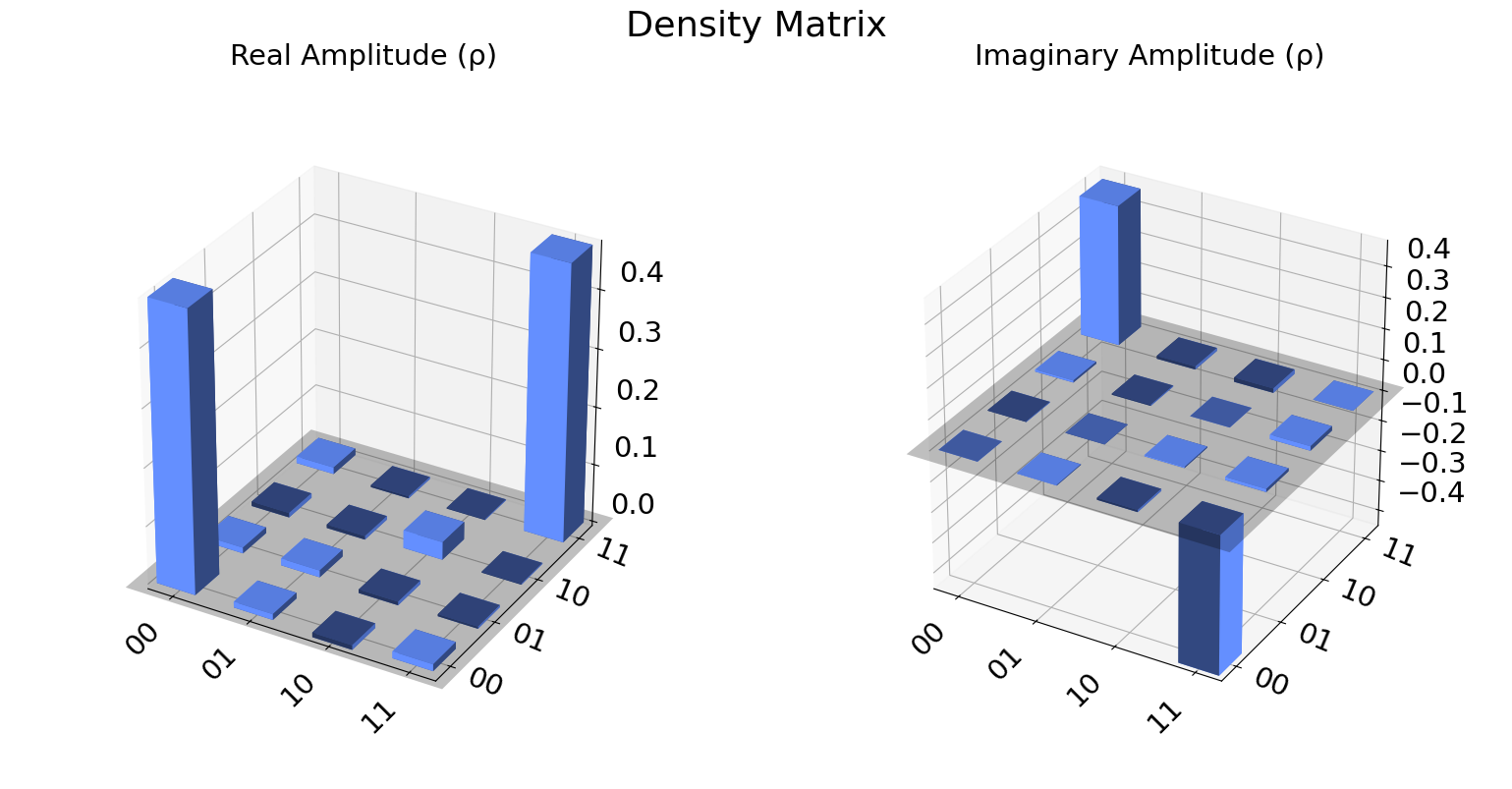
We can also visualize the density matrix:
from qiskit.visualization import plot_state_city
plot_state_city(qstdata1.analysis_results("state").value, title='Density Matrix')
The state fidelity of the fitted state with the ideal state prepared by
the input circuit is stored in the "state_fidelity" result field.
Note that if the input circuit contained any measurements the ideal
state cannot be automatically generated and this field will be set to
None.
fid_result = qstdata1.analysis_results("state_fidelity")
print("State Fidelity = {:.5f}".format(fid_result.value))
State Fidelity = 0.93136
Additional state metadata
Additional data is stored in the tomography under the
"state_metadata" field. This includes
eigvals: the eigenvalues of the fitted statetrace: the trace of the fitted statepositive: Whether the eigenvalues are all non-negativepositive_delta: the deviation from positivity given by 1-norm of negative eigenvalues.
If trace rescaling was performed this dictionary will also contain a raw_trace field
containing the trace before rescaling. Futhermore, if the state was rescaled to be
positive or trace 1 an additional field raw_eigvals will contain the state
eigenvalues before rescaling was performed.
state_result.extra
{'trace': 1.0000000000000016,
 'eigvals': array([0.9318245 , 0.03677227, 0.03140323, 0.        ]),
 'raw_eigvals': array([ 0.93259841,  0.03754617,  0.03217713, -0.00232171]),
 'rescaled_psd': True,
 'fitter_metadata': {'fitter': 'linear_inversion',
  'fitter_time': 0.007808208465576172},
 'conditional_probability': 1.0,
 'positive': True,
 'experiment': 'StateTomography',
 'run_time': None}
To see the effect of rescaling, we can perform a “bad” fit with very low counts:
# QST Experiment
bad_data = qstexp1.run(backend, shots=10, seed_simulation=100).block_for_results()
bad_state_result = bad_data.analysis_results("state")

# Print result
print(bad_state_result)

# Show extra data
bad_state_result.extra
AnalysisResult
- name: state
- value: DensityMatrix([[ 0.39987187+0.j        , -0.03552618+0.08697054j,
                 0.01794438-0.02263301j,  0.06851842-0.39181533j],
               [-0.03552618-0.08697054j,  0.09313915+0.j        ,
                 0.02742535+0.01701758j, -0.01238938+0.01480891j],
               [ 0.01794438+0.02263301j,  0.02742535-0.01701758j,
                 0.02332883+0.j        ,  0.06158607-0.03713812j],
               [ 0.06851842+0.39181533j, -0.01238938-0.01480891j,
                 0.06158607+0.03713812j,  0.48366015+0.j        ]],
              dims=(2, 2))
- quality: unknown
- extra: <9 items>
- device_components: ['Q0', 'Q1']
- verified: False
{'trace': 1.0,
 'eigvals': array([0.85494055, 0.14505945, 0.        , 0.        ]),
 'raw_eigvals': array([ 0.98023485,  0.27035376,  0.01451916, -0.26510776]),
 'rescaled_psd': True,
 'fitter_metadata': {'fitter': 'linear_inversion',
  'fitter_time': 0.0049440860748291016},
 'conditional_probability': 1.0,
 'positive': True,
 'experiment': 'StateTomography',
 'run_time': None}
Tomography Fitters
The default fitters is linear_inversion, which reconstructs the
state using dual basis of the tomography basis. This will typically
result in a non-positive reconstructed state. This state is rescaled to
be positive-semidefinite (PSD) by computing its eigen-decomposition and
rescaling its eigenvalues using the approach from Ref. [1].
There are several other fitters are included (See API documentation for
details). For example, if cvxpy is installed we can use the
cvxpy_gaussian_lstsq() fitter, which allows constraining the fit to be
PSD without requiring rescaling.
try:
    import cvxpy

    # Set analysis option for cvxpy fitter
    qstexp1.analysis.set_options(fitter='cvxpy_gaussian_lstsq')

    # Re-run experiment
    qstdata2 = qstexp1.run(backend, seed_simulation=100).block_for_results()

    state_result2 = qstdata2.analysis_results("state")
    print(state_result2)
    print("\nextra:")
    for key, val in state_result2.extra.items():
        print(f"- {key}: {val}")

except ModuleNotFoundError:
    print("CVXPY is not installed")
AnalysisResult
- name: state
- value: DensityMatrix([[ 0.49065344+0.j        ,  0.00067023+0.021021j  ,
                -0.01433498+0.00964313j, -0.00754156-0.44304552j],
               [ 0.00067023-0.021021j  ,  0.01756754+0.j        ,
                 0.00167635+0.01177565j,  0.01027588-0.01006195j],
               [-0.01433498-0.00964313j,  0.00167635-0.01177565j,
                 0.02600303+0.j        , -0.00894755-0.01886131j],
               [-0.00754156+0.44304552j,  0.01027588+0.01006195j,
                -0.00894755+0.01886131j,  0.46577598+0.j        ]],
              dims=(2, 2))
- quality: unknown
- extra: <9 items>
- device_components: ['Q0', 'Q1']
- verified: False

extra:
- trace: 1.0000000019246675
- eigvals: [9.21825627e-01 6.73481032e-02 1.08106510e-02 1.56188084e-05]
- raw_eigvals: [9.21825625e-01 6.73481031e-02 1.08106510e-02 1.56188084e-05]
- rescaled_psd: False
- fitter_metadata: {'fitter': 'cvxpy_gaussian_lstsq', 'cvxpy_solver': 'SCS', 'cvxpy_status': ['optimal'], 'psd_constraint': True, 'trace_preserving': True, 'fitter_time': 0.022126197814941406}
- conditional_probability: 1.0
- positive: True
- experiment: StateTomography
- run_time: None
Parallel Tomography Experiment
We can also use the ParallelExperiment class to
run subsystem tomography on multiple qubits in parallel.
For example if we want to perform 1-qubit QST on several qubits at once:
from math import pi
num_qubits = 5
gates = [qiskit.circuit.library.RXGate(i * pi / (num_qubits - 1))
         for i in range(num_qubits)]

subexps = [
    StateTomography(gate, physical_qubits=(i,))
    for i, gate in enumerate(gates)
]
parexp = ParallelExperiment(subexps)
pardata = parexp.run(backend, seed_simulation=100).block_for_results()

for result in pardata.analysis_results():
    print(result)
View component experiment analysis results:
for i, expdata in enumerate(pardata.child_data()):
    state_result_i = expdata.analysis_results("state")
    fid_result_i = expdata.analysis_results("state_fidelity")

    print(f'\nPARALLEL EXP {i}')
    print("State Fidelity: {:.5f}".format(fid_result_i.value))
    print("State: {}".format(state_result_i.value))
PARALLEL EXP 0
State Fidelity: 0.98340
State: DensityMatrix([[0.98339844+0.j        , 0.02734375+0.03027344j],
               [0.02734375-0.03027344j, 0.01660156+0.j        ]],
              dims=(2,))

PARALLEL EXP 1
State Fidelity: 0.97923
State: DensityMatrix([[0.84863281+0.j        , 0.01367188+0.32910156j],
               [0.01367188-0.32910156j, 0.15136719+0.j        ]],
              dims=(2,))

PARALLEL EXP 2
State Fidelity: 0.98340
State: DensityMatrix([[ 0.52246094+0.j        , -0.01171875+0.48339844j],
               [-0.01171875-0.48339844j,  0.47753906+0.j        ]],
              dims=(2,))

PARALLEL EXP 3
State Fidelity: 0.98199
State: DensityMatrix([[ 0.15722656+0.j        , -0.01953125+0.33886719j],
               [-0.01953125-0.33886719j,  0.84277344+0.j        ]],
              dims=(2,))

PARALLEL EXP 4
State Fidelity: 0.96973
State: DensityMatrix([[ 0.03027344+0.j        , -0.0078125 +0.00097656j],
               [-0.0078125 -0.00097656j,  0.96972656+0.j        ]],
              dims=(2,))
References
See also
API documentation:
StateTomography