Note

This is the documentation for the current state of the development branch of Qiskit Experiments. The documentation or APIs here can change prior to being released.

Getting Started

Installation

Qiskit Experiments is built on top of Qiskit, so we recommend that you first install Qiskit following its installation guide. Qiskit Experiments supports the same platforms and Python versions (currently 3.7+) as Qiskit itself.

Qiskit Experiments releases can be installed via the Python package manager pip in your shell environment:

python -m pip install qiskit-experiments

If you want to run the most up-to-date version instead (may not be stable), you can install the latest main branch:

python -m pip install git+https://github.com/Qiskit/qiskit-experiments.git

If you want to develop the package, you can install Qiskit Experiments from source by cloning the repository:

git clone https://github.com/Qiskit/qiskit-experiments.git
python -m pip install -e qiskit-experiments

The -e option will keep your installed package up to date as you make or pull new changes.

Running your first experiment

Let’s run a T1 Experiment, which estimates the characteristic relaxation time of a qubit from the excited state to the ground state, also known as $T_1$, by measuring the excited state population after varying delays. First, we have to import the experiment from the Qiskit Experiments library:

from qiskit_experiments.library import T1

Experiments must be run on a backend. We’re going to use a simulator, FakePerth, for this example, but you can use any backend, real or simulated, that you can access through Qiskit.

Note

This tutorial requires the qiskit-aer package to run simulations. You can install it with python -m pip install qiskit-aer.

from qiskit.providers.fake_provider import FakePerth
from qiskit_aer import AerSimulator

backend = AerSimulator.from_backend(FakePerth())

All experiments require a physical_qubits parameter as input that specifies which physical qubit or qubits the circuits will be executed on. The qubits must be given as a Python sequence (usually a tuple or a list).

Note

Since 0.5.0, using qubits instead of physical_qubits or specifying an integer qubit index instead of a one-element sequence for a single-qubit experiment is deprecated.

In addition, the $T_1$ experiment has a second required parameter, delays, which is a list of times in seconds at which to measure the excited state population. In this example, we’ll run the $T_1$ experiment on qubit 0, and use the t1 backend property of this qubit to give us a good estimate for the sweep range of the delays.

import numpy as np

qubit0_t1 = FakePerth().qubit_properties(0).t1
delays = np.arange(1e-6, 3 * qubit0_t1, 3e-5)

exp = T1(physical_qubits=(0,), delays=delays)

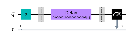
The circuits encapsulated by the experiment can be accessed using the experiment’s circuits() method, which returns a list of circuits that can be run on a backend. Let’s print the range of delay times we’re sweeping over and draw the first and last circuits for our $T_1$ experiment:

print(delays)
exp.circuits()[0].draw(output='mpl')

[1.00e-06 3.10e-05 6.10e-05 9.10e-05 1.21e-04 1.51e-04 1.81e-04 2.11e-04
 2.41e-04 2.71e-04 3.01e-04 3.31e-04 3.61e-04 3.91e-04 4.21e-04 4.51e-04
 4.81e-04 5.11e-04 5.41e-04 5.71e-04 6.01e-04]

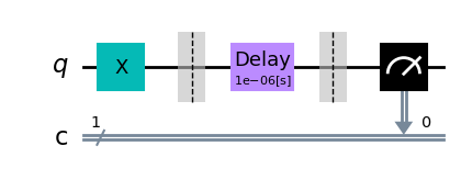
exp.circuits()[-1].draw(output='mpl')

As expected, the delay block spans the full range of time values that we specified.

The ExperimentData class

After instantiating the experiment, we run the experiment by calling run() with our backend of choice. This transpiles our experiment circuits then packages them into jobs that are run on the backend.

Note

See the how-tos for customizing job splitting when running an experiment.

This statement returns the ExperimentData class containing the results of the experiment, so it’s crucial that we assign the output to a data variable. We could have also provided the backend at the instantiation of the experiment, but specifying the backend at run time allows us to run the same exact experiment on different backends should we choose to do so.

exp_data = exp.run(backend=backend).block_for_results()

The block_for_results() method is optional and is used to block execution of subsequent code until the experiment has fully completed execution and analysis. If

exp_data = exp.run(backend=backend)

is executed instead, the statement will finish running as soon as the jobs are submitted, but the analysis callback won’t populate exp_data with results until the entire process has finished. In this case, there are two useful methods in the ExperimentData, job_status() and analysis_status(), that return the current status of the job and analysis, respectively:

print(exp_data.job_status())
print(exp_data.analysis_status())

JobStatus.DONE
AnalysisStatus.DONE

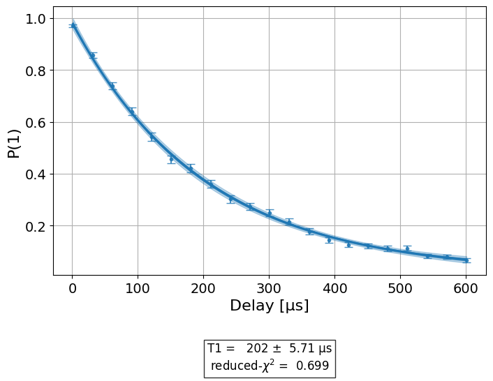
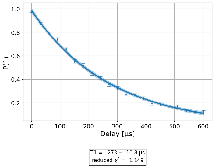
Once the analysis is complete, figures are retrieved using the figure() method. See the visualization module tutorial on how to customize figures for an experiment. For our $T_1$ experiment, we have a single figure showing the raw data and fit to the exponential decay model of the $T_1$ experiment:

display(exp_data.figure(0))

The fit results and associated parameters are accessed with analysis_results():

for result in exp_data.analysis_results():
    print(result)

AnalysisResult
- name: @Parameters_T1Analysis
- value: CurveFitResult:
 - fitting method: least_squares
 - number of sub-models: 1
  * F_exp_decay(x) = amp * exp(-x/tau) + base
 - success: True
 - number of function evals: 24
 - degree of freedom: 18
 - chi-square: 12.581906158016226
 - reduced chi-square: 0.698994786556457
 - Akaike info crit.: -4.757516175730618
 - Bayesian info crit.: -1.6239488625603489
 - init params:
  * amp = 0.9034146341463414
  * tau = 0.00022477245253449803
  * base = 0.06682926829268293
 - fit params:
  * amp = 0.9617947020071678 ± 0.008604532199225402
  * tau = 0.00020165363923484243 ± 5.707813625419415e-06
  * base = 0.020040925777814807 ± 0.00782960614706135
 - correlations:
  * (tau, base) = -0.9011491629801396
  * (amp, base) = -0.6201314853157044
  * (amp, tau) = 0.37961569467819706
- quality: good
- device_components: ['Q0']
- verified: False
AnalysisResult
- name: T1
- value: 0.000202+/-0.000006
- χ²: 0.698994786556457
- quality: good
- extra: <1 items>
- device_components: ['Q0']
- verified: False

Results can be indexed numerically (starting from 0) or using their name.

Note

See the analysis_results() API documentation for more advanced usage patterns to access subsets of analysis results.

Each analysis result value is a UFloat object from the uncertainties package. The nominal value and standard deviation of each value can be accessed as follows:

print(exp_data.analysis_results("T1").value.nominal_value)
print(exp_data.analysis_results("T1").value.std_dev)

0.00020165363923484243
5.707813625419415e-06

For further documentation on how to work with UFloats, consult the uncertainties User Guide.

Raw circuit output data and its associated metadata can be accessed with the data() property. Data is indexed by the circuit it corresponds to. Depending on the measurement level set in the experiment, the raw data will either be in the key counts (level 2) or memory (level 1 IQ data).

Note

See the data processor tutorial for more information on level 1 and level 2 data.

Circuit metadata contains information set by the experiment on a circuit-by-circuit basis; xval is used by the analysis to extract the x value for each circuit when fitting the data.

print(exp_data.data(0))

{'counts': {'0': 30, '1': 994}, 'job_id': '708c0c1f-5502-41c4-8c08-350b7c9a69f4', 'metadata': {'experiment_type': 'T1', 'qubit': 0, 'unit': 's', 'xval': 1e-06}, 'shots': 1024, 'meas_level': <MeasLevel.CLASSIFIED: 2>}

Experiments also have global associated metadata accessed by the metadata() property.

print(exp_data.metadata)

{'physical_qubits': [0], 'meas_level': <MeasLevel.CLASSIFIED: 2>, '_source': {'class': 'qiskit_experiments.framework.experiment_data.ExperimentData', 'metadata_version': 1, 'qiskit_version': '0.43.3'}}

The actual backend jobs that were executed for the experiment can be accessed with the jobs() method.

Note

See the how-tos for rerunning the analysis for an existing experiment that finished execution.

Setting options for your experiment

It’s often insufficient to run an experiment with only its default options. There are four types of options one can set for an experiment:

Run options

These options are passed to the experiment’s run() method and then to the run() method of your specified backend. Any run option that your backend supports can be set:

from qiskit.qobj.utils import MeasLevel

exp.set_run_options(shots=1000,
                    meas_level=MeasLevel.CLASSIFIED)

Consult the documentation of the run method of your specific backend type for valid options. For example, see qiskit_ibm_provider.IBMBackend.run() for IBM backends.

Transpile options

These options are passed to the Terra transpiler to transpile the experiment circuits before execution:

exp.set_transpile_options(scheduling_method='asap',
                          optimization_level=3,
                          basis_gates=["x", "sx", "rz"])

Consult the documentation of qiskit.compiler.transpile() for valid options.

Experiment options

These options are unique to each experiment class. Many experiment options can be set upon experiment instantiation, but can also be explicitly set via set_experiment_options():

exp = T1(physical_qubits=(0,), delays=delays)
new_delays=np.arange(1e-6, 600e-6, 50e-6)
exp.set_experiment_options(delays=new_delays)

Consult the API documentation for the options of each experiment class.

Analysis options

These options are unique to each analysis class. Unlike the other options, analyis options are not directly set via the experiment object but use instead a method of the associated analysis:

from qiskit_experiments.library import StandardRB

exp = StandardRB(physical_qubits=(0,),
                lengths=list(range(1, 300, 30)),
                seed=123,
                backend=backend)
exp.analysis.set_options(gate_error_ratio=None)

Consult the API documentation for the options of each experiment’s analysis class.

Running experiments on multiple qubits

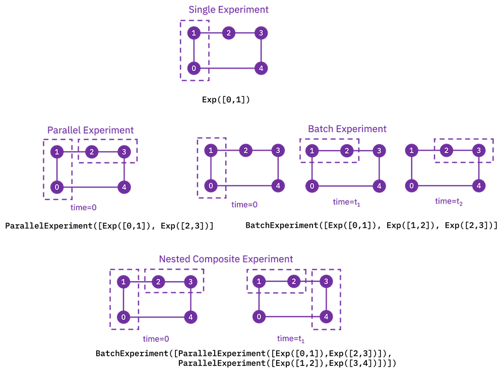
To run experiments across many qubits of the same device, we use composite experiments. A composite experiment is a parent object that contains one or more child experiments, which may themselves be composite. There are two core types of composite experiments:

• Parallel experiments run across qubits simultaneously as set by the user. The circuits of child experiments are combined into new circuits that map circuit gates onto qubits in parallel. Therefore, the circuits in child experiments cannot overlap in the physical_qubits parameter. The marginalization of measurement data for analysis of each child experiment is handled automatically.

• Batch experiments run consecutively in time. These child circuits can overlap in qubits used.

Using parallel experiments, we can measure the $T_1$ of one qubit while doing a standard Randomized Benchmarking StandardRB experiment on other qubits simultaneously on the same device:

from qiskit_experiments.framework import ParallelExperiment

child_exp1 = T1(physical_qubits=(2,), delays=delays)
child_exp2 = StandardRB(physical_qubits=(3,1), lengths=np.arange(1,100,10), num_samples=2)
parallel_exp = ParallelExperiment([child_exp1, child_exp2])

Note that when the transpile and run options are set for a composite experiment, the child experiments’s options are also set to the same options recursively. Let’s examine how the parallel experiment is constructed by visualizing child and parent circuits. The child experiments can be accessed via the component_experiment() method, which indexes from zero:

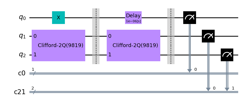
parallel_exp.component_experiment(0).circuits()[0].draw(output='mpl')

parallel_exp.component_experiment(1).circuits()[0].draw(output='mpl')

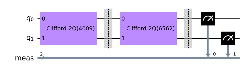
The circuits of all experiments assume they’re acting on virtual qubits starting from index 0. In the case of a parallel experiment, the child experiment circuits are composed together and then reassigned virtual qubit indices:

parallel_exp.circuits()[0].draw(output='mpl')

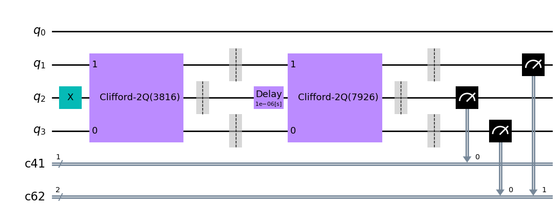
During experiment transpilation, a mapping is performed to place these circuits on the physical layout. We can see its effects by looking at the transpiled circuit, which is accessed via the internal method _transpiled_circuits(). After transpilation, the T1 experiment is correctly placed on physical qubit 2 and the StandardRB experiment’s gates are on physical qubits 3 and 1.

parallel_exp._transpiled_circuits()[0].draw(output='mpl')

ParallelExperiment and BatchExperiment classes can also be nested arbitrarily to make complex composite experiments.

Viewing child experiment data

The experiment data returned from a composite experiment contains individual analysis results for each child experiment that can be accessed using child_data(). By default, the parent data object does not contain analysis results.

parallel_data = parallel_exp.run(backend, seed_simulator=101).block_for_results()

for i, sub_data in enumerate(parallel_data.child_data()):
    print("Component experiment",i)
    display(sub_data.figure(0))
    for result in sub_data.analysis_results():
        print(result)

Component experiment 0

AnalysisResult
- name: @Parameters_T1Analysis
- value: CurveFitResult:
 - fitting method: least_squares
 - number of sub-models: 1
  * F_exp_decay(x) = amp * exp(-x/tau) + base
 - success: True
 - number of function evals: 20
 - degree of freedom: 18
 - chi-square: 20.683976293629215
 - reduced chi-square: 1.149109794090512
 - Akaike info crit.: 5.681574284462717
 - Bayesian info crit.: 8.815141597632985
 - init params:
  * amp = 0.8595121951219512
  * tau = 0.00027484081394614214
  * base = 0.11560975609756098
 - fit params:
  * amp = 0.9852558029201177 ± 0.013335251509204699
  * tau = 0.0002732697700337059 ± 1.0771661158575468e-05
  * base = 0.00017910642718570646 ± 0.014919371946027101
 - correlations:
  * (tau, base) = -0.9495837058208386
  * (amp, base) = -0.8546234501452962
  * (amp, tau) = 0.7124235042569481
- quality: good
- device_components: ['Q2']
- verified: False
AnalysisResult
- name: T1
- value: 0.000273+/-0.000011
- χ²: 1.149109794090512
- quality: good
- extra: <1 items>
- device_components: ['Q2']
- verified: False
Component experiment 1

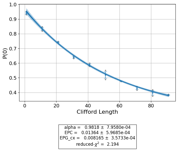
AnalysisResult
- name: @Parameters_RBAnalysis
- value: CurveFitResult:
 - fitting method: least_squares
 - number of sub-models: 1
  * F_rb_decay(x) = a * alpha ** x + b
 - success: True
 - number of function evals: 20
 - degree of freedom: 7
 - chi-square: 15.356995252864428
 - reduced chi-square: 2.1938564646949184
 - Akaike info crit.: 10.28985994030782
 - Bayesian info crit.: 11.19761521928996
 - init params:
  * a = 0.7042717262167281
  * alpha = 0.981813395162991
  * b = 0.25
 - fit params:
  * a = 0.7226167320532181 ± 0.010946487458703958
  * alpha = 0.9818166767769019 ± 0.0007958048775382812
  * b = 0.243304015947197 ± 0.01374474957040744
 - correlations:
  * (alpha, b) = -0.9701584971758207
  * (a, b) = -0.8691412248895404
  * (a, alpha) = 0.7497140621121863
- quality: good
- device_components: ['Q3', 'Q1']
- verified: False
AnalysisResult
- name: alpha
- value: 0.9818+/-0.0008
- χ²: 2.1938564646949184
- quality: good
- device_components: ['Q3', 'Q1']
- verified: False
AnalysisResult
- name: EPC
- value: 0.0136+/-0.0006
- χ²: 2.1938564646949184
- quality: good
- device_components: ['Q3', 'Q1']
- verified: False
AnalysisResult
- name: EPG_cx
- value: 0.0082+/-0.0004
- χ²: 2.1938564646949184
- quality: good
- device_components: ['Q3', 'Q1']
- verified: False

If you want the parent data object to contain the analysis results instead, you can set the flatten_results flag to true to flatten the results of all component experiments into one level:

parallel_exp = ParallelExperiment(
    [T1(physical_qubits=(i,), delays=delays) for i in range(2)], flatten_results=True
)
parallel_data = parallel_exp.run(backend, seed_simulator=101).block_for_results()

for result in parallel_data.analysis_results():
    print(result)

AnalysisResult
- name: @Parameters_T1Analysis
- value: CurveFitResult:
 - fitting method: least_squares
 - number of sub-models: 1
  * F_exp_decay(x) = amp * exp(-x/tau) + base
 - success: True
 - number of function evals: 20
 - degree of freedom: 18
 - chi-square: 16.777233960918313
 - reduced chi-square: 0.9320685533843507
 - Akaike info crit.: 1.2855085743960357
 - Bayesian info crit.: 4.419075887566305
 - init params:
  * amp = 0.8868292682926829
  * tau = 0.00022717300819969968
  * base = 0.07560975609756097
 - fit params:
  * amp = 0.9591563783072699 ± 0.008722718232923832
  * tau = 0.00020563098809331363 ± 5.916681239621023e-06
  * base = 0.01817301256948842 ± 0.008075085380244483
 - correlations:
  * (tau, base) = -0.9053821521891239
  * (amp, base) = -0.6352894942116918
  * (amp, tau) = 0.40113906329346544
- quality: good
- extra: <1 items>
- device_components: ['Q0']
- verified: False
AnalysisResult
- name: T1
- value: 0.000206+/-0.000006
- χ²: 0.9320685533843507
- quality: good
- extra: <2 items>
- device_components: ['Q0']
- verified: False
AnalysisResult
- name: @Parameters_T1Analysis
- value: CurveFitResult:
 - fitting method: least_squares
 - number of sub-models: 1
  * F_exp_decay(x) = amp * exp(-x/tau) + base
 - success: True
 - number of function evals: 21
 - degree of freedom: 18
 - chi-square: 16.854244267918833
 - reduced chi-square: 0.9363469037732686
 - Akaike info crit.: 1.3816815265654254
 - Bayesian info crit.: 4.515248839735695
 - init params:
  * amp = 0.9356097560975609
  * tau = 0.0001858364229100068
  * base = 0.042439024390243905
 - fit params:
  * amp = 0.969314571640488 ± 0.006775226516899206
  * tau = 0.00017009353906185276 ± 3.810457000354833e-06
  * base = 0.011497161200531443 ± 0.005000160772463704
 - correlations:
  * (tau, base) = -0.8566281535749727
  * (amp, base) = -0.5169272804382684
  * (amp, tau) = 0.2538512206205129
- quality: good
- extra: <1 items>
- device_components: ['Q1']
- verified: False
AnalysisResult
- name: T1
- value: 0.000170+/-0.000004
- χ²: 0.9363469037732686
- quality: good
- extra: <2 items>
- device_components: ['Q1']
- verified: False