Solving the Schrodinger equation with either NumPy or JAX using the default NumPy alias

In this tutorial, we will learn how to write generic code with examples of numerical computation by using NumPy and JAX. We’ll use a code example that employs the Runge-Kutta method to numerically simulate the matrix evolution of the Schrodinger equation. In addition, we will show how to add new dispatched function to Alias instance using Alias.register_function().

In this section, we will go through the following steps:

1. Import the required libraries and initialize the default NumPy alias.

2. Define a function for evaluating the right-hand side of the Schrodinger equation using the default NumPy alias.

3. Solve the Schrodinger equation using the right-hand side function and existing NumPy-based and JAX-based solvers.

4. Register new dispatched custom solvers using Alias.register_function() method.

5. Solve the Schrodinger equation using the custom solvers.

1. Import the required libraries and initialize the default NumPy alias

Here, we import the necessary libraries.

from arraylias import numpy_alias
import numpy as np
import matplotlib.pyplot as plt
import jax
import jax.numpy as jnp

jax.config.update("jax_enable_x64", True)
jax.config.update("jax_platform_name", "cpu")

from scipy.integrate import solve_ivp
from jax.experimental.ode import odeint

# set some variables
dt = 0.01
N = 1001

Initialize the default NumPy alias.

alias = numpy_alias()
unp = alias()

2. Define a function for evaluating the right-hand side of the Schrodinger equation using the default NumPy alias

We solve the Schrodinger equation using the Runge-Kutta method in this tutorial. The Schrodinger equation is the differential equation

\[\psi'(t) = -i * H(t) \psi(t),\]

where \(H(t)\) is a time-dependent matrix called the Hamiltonian, and \(\psi(t)\) is the state of the system.

We will solve a common model for a two-level quantum system, which has Hamiltonian

\[H(t) = \times 2 \pi \nu_z \frac{Z}{2} + 2 \pi \nu_x \cos(2 \pi \nu_d t)\frac{X}{2},\]

where \(\{X,Y,Z\}\) are the Pauli matrices, and \(\nu_z\), \(\nu_x\), and \(\nu_d\) are model parameters of the system.

Write a function representing the right-hand side of the Schrodinger equation with the above Hamiltonian.

Z = np.array([[1, 0], [0, -1]])
X = np.array([[0, 1], [1, 0]])


def rhs(t, y):
    return unp.matmul(-1j * (5 * Z - unp.cos(10 * t) * X), y)

Depending on the input type, the rhs function will execute using either NumPy or JAX, which we can confirm by observing the output types:

# Numpy input
rhs(0.1, np.array([0.0, 1.0]))

array([0.+0.54030231j, 0.+5.j        ])

# Jax.numpy input
rhs(jnp.array(0.1), jnp.array([0.0, 1.0]))

Array([0.+0.54030231j, 0.+5.j        ], dtype=complex128)

Define a function for computing the probability of observing the system in a given state to be used throughout the tutorial:

def state_probabilities(state):
    return unp.abs(state) ** 2

3. Solve the Schrodinger equation using the right-hand side function and existing NumPy-based and JAX-based solvers

Here we show how the rhs function can be passed to numerical ODE solvers in both SciPy and JAX as if the function had been natively written in either library.

First, we solve the equation by using NumPy as the input and scipy.integrate.solve_ivp as a solver. We define the initial state, the time span for the simulation, and time point we want to simulate.

init_state = np.array([1.0 + 0j, 0.0 + 0j])

t_span = [0, (N - 1) * dt]
T = np.linspace(0, (N - 1) * dt, N)

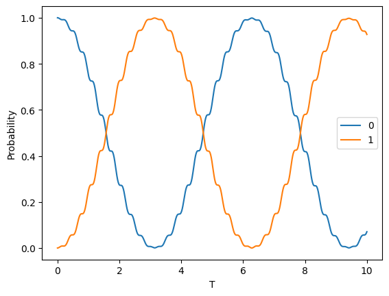
We solve by using scipy.integrate.solve_ivp and plot the probabilities of each state.

sol = solve_ivp(rhs, t_span, init_state, method="RK45", t_eval=T)
probabilities = state_probabilities(sol.y)

plt.plot(sol.t, probabilities[0], label="0")
plt.plot(sol.t, probabilities[1], label="1")
plt.xlabel("T")
plt.ylabel("Probability")
plt.legend()
plt.show()

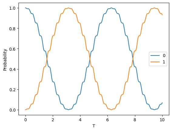
Second, we solve the equation by using jax.numpy.array as the input and jax.experimental.ode.odeint as a solver.

init_state = jnp.array([1.0 + 0j, 0.0 + 0j])

t_span = [0, (N - 1) * dt]
T = jnp.linspace(0, (N - 1) * dt, N)

sol = odeint(lambda y, t: rhs(t, y), init_state, T)
probabilities = state_probabilities(sol.T)
plt.plot(T, probabilities[0], label="0")
plt.plot(T, probabilities[1], label="1")
plt.xlabel("T")
plt.ylabel("Probability")
plt.legend()
plt.show()

4. Register new dispatched custom solvers using Alias.register_function() method

In this section, we define custom functions for solving differential equations in both NumPy and JAX, and register them to our instance of the NumPy alias.

We will use the 4th order Runge-Kutta method, whose single step formula is:

\[\begin{split}k_1 &= h \cdot f(t_n, y_n) \\ k_2 &= h \cdot f(t_n + \frac{h}{2}, y_n + \frac{k_1}{2}) \\ k_3 &= h \cdot f(t_n + \frac{h}{2}, y_n + \frac{k_2}{2}) \\ k_4 &= h \cdot f(t_n + h, y_n + k_3) \\ y_{n+1} &= y_n + \frac{1}{6}(k_1 + 2k_2 + 2k_3 + k_4)\end{split}\]

where \(y_{n}\), \(t_{n}\), and \(h\) are current solution, current time, and time step size, respectively.

Define a function for taking a single Runge-Kutta step:

def runge_kutta_step(t, y, dt, rhs):
    k1 = dt * rhs(t, y)
    k2 = dt * rhs(t + 0.5 * dt, y + 0.5 * k1)
    k3 = dt * rhs(t + 0.5 * dt, y + 0.5 * k2)
    k4 = dt * rhs(t + dt, y + k3)
    return (k1 + 2 * k2 + 2 * k3 + k4) / 6.0

First, define the version of the solver written for use with standard NumPy, and register it to our alias instance to act on NumPy arrays using alias.register_function:

@alias.register_function(lib="numpy", path="runge_kutta")
def _(y0, dt, N, rhs):
    probabilities = []
    for n in range(N):
        probabilities.append(state_probabilities(y0))
        y0 += runge_kutta_step(n * dt, y0, dt, rhs)
    return probabilities

Next, register a version of the solver to work on JAX arrays. For better behaviour under JAX transformations, we need to use the JAX looping construct jax.lax.scan rather than the standard Python for loop:

@alias.register_function(lib="jax", path="runge_kutta")
def _(y0, dt, N, rhs):
    def runge_kutta_step_scan(carry, probabilities):
        n, y = carry
        probabilities = state_probabilities(y)
        y += runge_kutta_step(n * dt, y, dt, rhs)
        return (n + 1, y), probabilities

    _, probabilities = jax.lax.scan(runge_kutta_step_scan, (0, y0), jnp.zeros((N, 2)))
    return probabilities

5. Solve the Schrodinger equation using the custom solvers

Finally, we will solve the Schrodinger equation using both the NumPy and JAX libraries via our single dispatched function unp.runge_kutta.

First, solve with NumPy:

init_state = np.array([1.0 + 0j, 0.0 + 0j])

probabilities = unp.array(unp.runge_kutta(init_state, dt, N, rhs))

T = np.linspace(0, (N - 1) * dt, N)
plt.plot(T, probabilities, label=["0", "1"])
plt.xlabel("T")
plt.ylabel("Probability")
plt.legend()
plt.show()

%timeit unp.array(unp.runge_kutta(init_state, dt, N, rhs))

66 ms ± 299 µs per loop (mean ± std. dev. of 7 runs, 10 loops each)

Second case is JAX:

init_state = jnp.array([1.0 + 0j, 0.0 + 0j])
probabilities = unp.array(unp.runge_kutta(init_state, dt, N, rhs))

T = np.linspace(0, (N - 1) * dt, N)

plt.plot(T, probabilities, label=["0", "1"])
plt.xlabel("T")
plt.ylabel("Probability")
plt.legend()
plt.show()

Lastly, we verify that the function unp.runge_kutta behaves as expected under JAX transformations.

from functools import partial


@partial(jax.jit, static_argnums=(2, 3))
def solve_with_RungeKutta_jit(y, dt, N, rhs):
    return unp.array(unp.runge_kutta(y, dt, N, rhs))

%timeit solve_with_RungeKutta_jit(init_state, dt, N, rhs)

118 µs ± 764 ns per loop (mean ± std. dev. of 7 runs, 10,000 loops each)